Lecture 1: Introduction to Graphical Models

Introducing why graphical models are useful, and an overview of the main types of graphical models.

The Fundamental Questions of Graphical Modeling

A graphical model is a method of modeling a probability distribution for reasoning under uncertainty, which is needed in applications such as speech recognition and computer vision. We usually have a sample of data points: $D = {X_{1}^{(i)},X_{2}^{(i)},…,X_{m}^{(i)} }_{i=1}^N$. The relations of the components in each $X$ can be depicted using a graph $G$. We then have our model $M_G$.

A graph for a model

Graphical models allow us to address three fundamental questions:

1. How should I represent my data in a way that reflects domain knowledge while acknowledging uncertainty?
2. How do I make inferences from this data?
3. How can I learn the 'right' model for this data?

Each of these questions can be rephrased as a question about probability distributions:

1. What is the joint probability distribution over my input variables? Which state configurations of the distribution are actually relevant to the problem?
2. How can we obtain the state probabilities? Do we use maximum-likelihood estimation, or can we use domain knowledge?
3. How can we compute conditional distributions of unobserved (latent) variable without needing to sum over a large number of state configurations?

In the next section, we give an example to show how graphical models provide an effective way of answering these questions.

---

Structure within a Cell: real world example of graphical models with structure among the RVs

Cell Structure Example

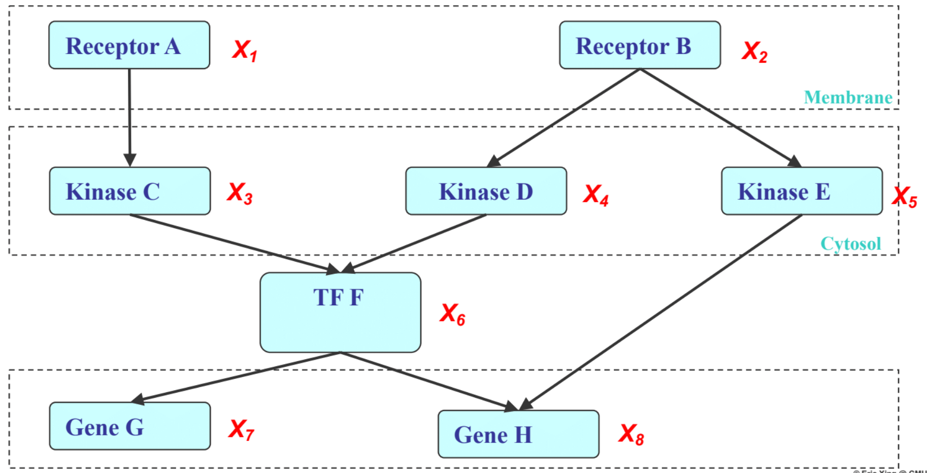
Receptors: Receive signal from cell surface

Kinase: Reads and decodes the signal

TF: Takes in the signal and triggers production of DNA with DNA template

Gene: DNA templates

We can incorporate such domain knowledge to impose structure on the RVs $X_{1},…,X_{8}$. A preliminary way is to partition the RV’s into compartments they reside in within a cell. Then we can model edges(pathway) that model the dependencies(communication) among the RVs(nodes).

With this structure, we can better express the joint probabilities among the RVs than with a full joint distribution table. The Factorization Law gives us a way to do so. The Factorization Law is a graph traversal algorithm that outputs a unique representation of the joint probability of the RVs. Concisely, we traverse the graph and identify the conditional probabilities of each node given its parent nodes and the marginal probabilities of nodes that do not have parents, then multiply all terms together for the joint probability of all nodes.

There are 3 main benefits of representing the joint distribution in this manner (with a graph structure and conditional probabilities that tie parent nodes and child nodes)

---

Three Main Benefits of Graphical Models

The first benefit is the cost savings in representing the joint distribution. By modeling the dependencies among the RVs with a graph and conditionals, the number of parameters needed to describe the joint distribution is much fewer than when using a full joint distribution table.

Assume all RVs are binary.

\begin{aligned} P(X_{1}) &\rightarrow 1\ \text{parameter} \\ P(X_{2}) &\rightarrow 1\ \text{parameter} \\ P(X_{3} \mid X_{1}) &\rightarrow 2\ \text{parameters} \\ P(X_{4} \mid X_{2}) &\rightarrow 2\ \text{parameters} \\ P(X_{5} \mid X_{2}) &\rightarrow 2\ \text{parameters} \\ P(X_{6} \mid X_{3}, X_{4}) &\rightarrow 4\ \text{parameters} \\ P(X_{7} \mid X_{6}) &\rightarrow 2\ \text{parameters} \\ P(X_{8} \mid X_{5}, X_{6}) &\rightarrow 4\ \text{parameters} \\ \end{aligned}

Thus, we have a total of 18 parameters.

Meanwhile, with a full joint distribution table, we would need $2^{8}-1$ parameters.

The second benefit is data integration. By factoring the joint distribution into modular terms, each term becomes self-contained and we can estimate each term with only the relevant data points (e.g. to estimate $P(X_{8}|X_{5}, X_{6})$ we only need data for $X_{8}, X_{5}, X_{6}$). Therefore, the problem of joint distribution estimation can be modularized into smaller pieces and integrated later by multiplication.

Examples:

• Cell molecules example
  • One lab can study the subtree formed by $X_{1}, X_{3}, X_{6}, X_{7}, X_{8}$ while another lab can study $X_{2}, X_{4}, X_{5}$, then fuse their estimations together by multiplying the terms by their dependencies.
• Cellphone usage
  • We can separately study the distribution represented by the user’s text, image and network data and fuse them together with a graphic model to derive the joint distribution.
• Genomics/biology
  • We routinely combine various data together with graphical models.

Finally, graphical models provide a generic method of representing knowledge and making inferences.

We can encode our domain knowledge through priors and incorporate them into our inference via the Bayes Theorem:

\begin{array}{rcl} p(h|d) &=& \frac{p(d|h)p(h)}{p(d)} \\ p(h|d) &=& \text{ posterior} \\ p(d|h) &=& \text{ likelihood} \\ p(h) &=& \text{ prior} \\ p(d) &=& \text{ marginal probability of the data}=\int_{H}p(d|h)p(h)dh \\ \end{array}

A graphical model provides a structured and efficient way for doing these computations. Therefore, a graphical model along with the Bayes Theorem provide a universal way of representing knowledge and computation.

---

PGM’s vs GM’s

Next, we will elaborate on the difference between Probabilistic Graphical Models (PGM) and Graphical Models (GM). In brief, a PGM adds structure to a multivariate statistical distribution, while a GM adds structure to any multivariate objective function.

A PGM minimizes the cost of designing a probability distribution. Formally, a PGM is a family of distributions over a given set of random variables. These distributions must be compatible with all the independence relationships among the variables, which are encoded in a graph.

In the graph itself, the type of edge used denotes the relationship among the variables. Directed edges denote causality, while undirected edges denote correlation.

Bayesian network A directed acyclic graph (DAG).

Markov random field An undirected graph.

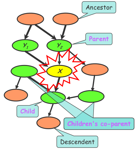
For instance, the Bayes net uses a directed acyclic graph (DAG). Each node in a Bayes net has a Markov blanket, composed of its parents, its children, and its children’s parents. Every node is conditionally independent of the nodes outside its Markov Blanket. Therefore, the local conditional probabilities as well as the graph structure completely determine the joint probability distribution. This model can be used to generate new data.

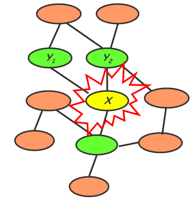
By contrast, the Markov random field uses an undirected graph. Every node is conditionally independent of the other graph nodes, except for its immediate neighbors. To determine the joint probability distribution, we need to know local contingency functions as well as structural cliques. This model cannot explicitly generate new data.

---

Equivalence Theorem / PGM Genealogy

We will be discussing the Equivalence Theorem, stated as follows:

For a graph $G$,

• Let $D_1$ denote the family of all distributions that satisfy $I(G)$,

• Let $D_2$ denote the family of all distributions that factor according to $G$,

then $D_1 \equiv D_2$.

The theorem is interpreted in two ways:

1. Separation properties in the graph imply independence properties about the associated variables.
2. For the graph to be useful, any conditional independence properties we can derive from the graph should hold for the probability distribution that the graph represents.

The study of Graphical Models involves the following parts:

1. Density estimation with parametric and nonparametric methods
2. Regression: linear, conditional mixture, nonparametric
3. Classification with generative and discriminative approaches
4. Clustering

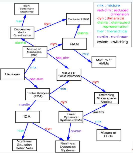
A partial genealogy of graphical models is as follows:

Genealogy of Graphical Models

---

Fancier GMs and Applications of GMs

GMs can be applied in numerous more advanced ways to solve complex problems in areas like reinforcement learning, machine translation, genetic pedigrees and solid state physics.

The applications of GMs include but are not limited to the following areas: Machine Learning, Computational Statistics, Computer Vision and Graphics, Natural Language Processing, Informational Retrieval, Robotic Control, etc.

Why should we study graphical models?

Design and analysis of algorithms in the fields of artificial intelligence, machine learning, natural language processing, etc. encounter issues like uncertainty and complexity. In graphical models, we use the idea of modularity, and view such complex problems as combinations of simpler parts. Tools from graphical models can be used for communication of information in networks. They can also be used to ease computation (simplify computational complexities and reduce time required for computations). As such, graphical model formalism can be used for development of efficient software packages for decision making and learning in problems rely on huge datasets.

Below we mention a few prominent reasons why one can use probabilistic graphical models:

• In graphical models, we break tasks into combinations of simpler parts. Probability theory helps to connect these simple parts with each other in a coherent and consistent manner.
• Graph theory gives an easy-to-understand interface in which models with multiple variables can be cast. Such interfaces help to uncover interactions, dependencies between difference sets of variables. As a consequence, graph theory also helps in the design of more efficient algorithms.
• Formalisms in general graphical model can be used for tasks in a plethora of fields like information theory, cyber security, systems engineering, pattern recognition etc.
• The generality of graphical model frameworks gives us a way to view different systems as occurrences of a common underlying formalism.

Plans for class

In this course, we will see an in-depth exploration of issues related to learning within the probabilistic graphical model formalism. The course will be divided into three main sections: Fundamentals of graphical models, advanced topics in graphical models, popular graphical models and applications. An outline of the topics that will be covered in this class is given below:

• Fundamentals of graphical models
  • Bayesian Network and Markov Random Fields
  • Discrete, Continuous and Hybrid models, Exponential family, Generalized Linear Models
  • Inference and Learning
• Advanced topics and latest developments in graphical models
  • Approximate inference
  • Infinite graphical models: nonparametric Bayesian models
  • Optimization-theoretic formulations for graphical models, e.g., Structured sparsity
  • Graphical models vs Deep nets
  • Nonparametric and spectral graphical models
  • Alternative graphical model learning paradigms
• Popular graphical models and applications
  • Multivariate gaussian models
  • Conditional random fields
  • Mixed-membership