Lecture 2: Bayesian Networks
Overview of Bayesian Networks, their properties, and how they can be helpful to model the joint probability distribution over a set of random variables. Concludes with a summary of relevant sections from the textbook reading.
Motivation: representing joint distributions over some random variables is computationally expensive, so we need methodologies to represent joint distributions compactly.
Two types of Graphical Models
Directed Graphs (Bayesian Networks)
An acyclic graph, $\mathcal{G}$, is made up of a set of nodes, $\mathcal{V}$, and a set of directed edges, $\mathcal{E}$, where edges represent a causality relationship between nodes. Nodes in the graph represent a set of random variables, ${X_1,…,X_N}$, where there is a one-to-one map between nodes and random variables.
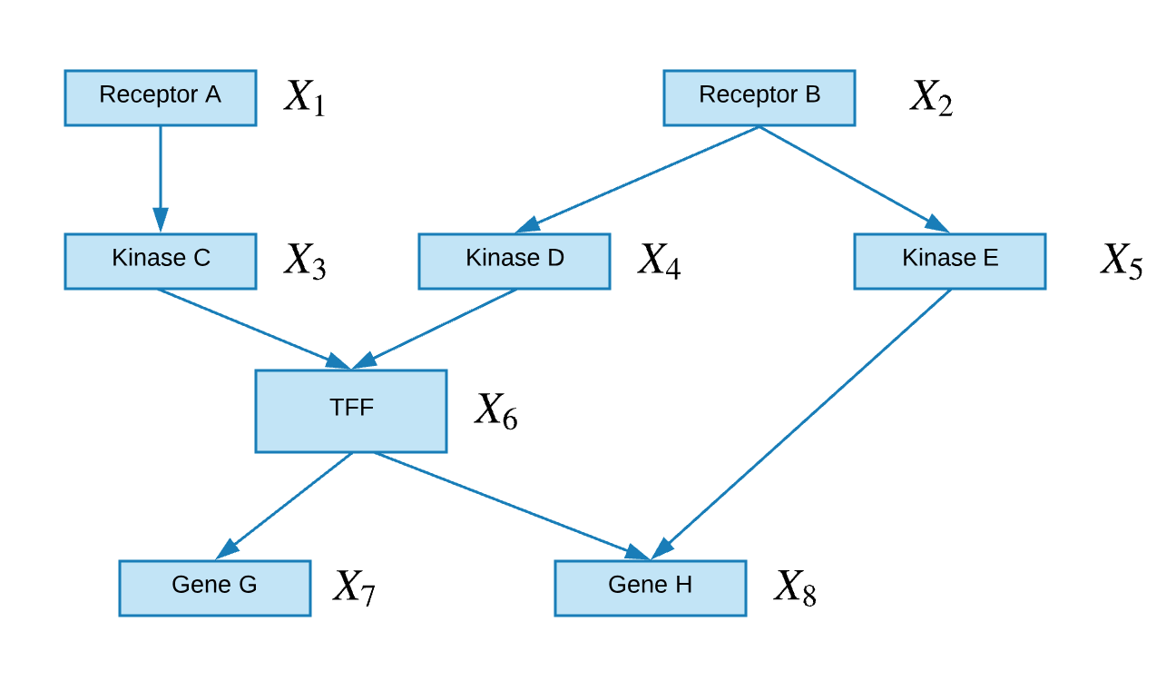
The joint probability of the above directed graph can be written as follows:
\[P(X_1, \dots ,X_8) = P(X_1)P(X_2)P(X_3|X_1)P(X_4|X_2)P(X_5|X_2)P(X_6|X_3,X_4)P(X_7|X_6)P(X_8|X_5,X_6)\]Undirected Graphs (Markov Random Fields)
An undirected graph contains nodes that are connected via non-directional edges.
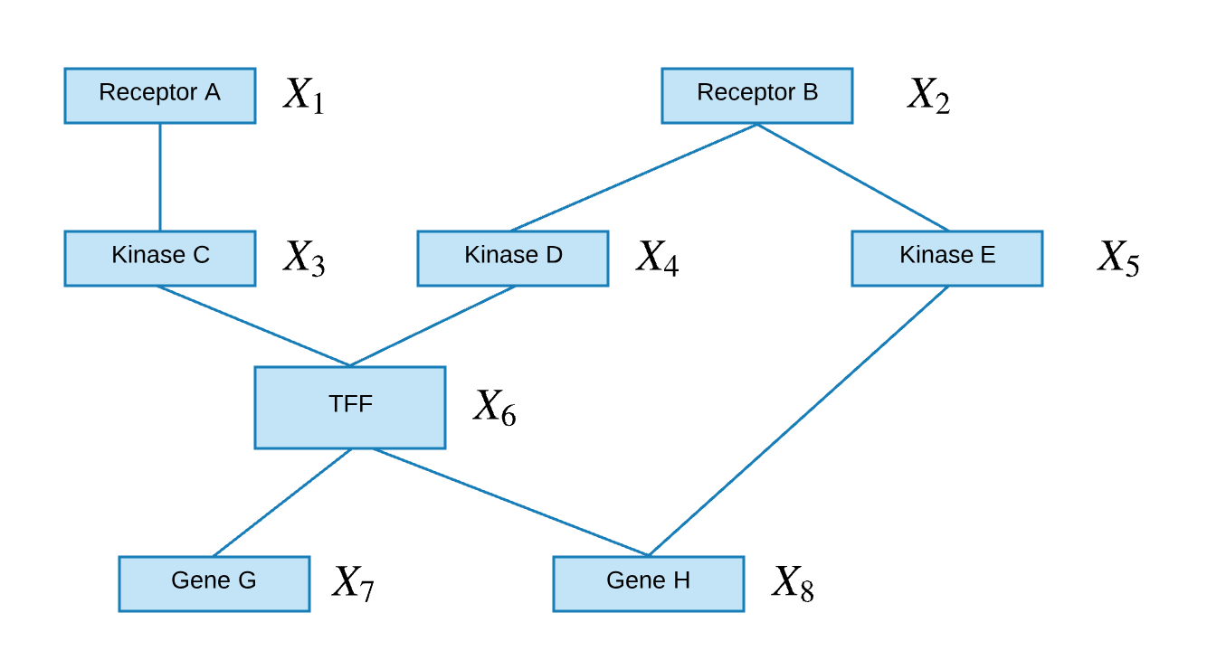
The joint probability of the above undirected graph can be written as followed:
Notation
- Variable: capitalized english letter, with subscripts to represent dimensions $(i, j, k)$ and superscripts to represent index e.g. $V_{i, j}^j$.
- Values of variables: a lowercase letter means it is an ‘observed value’ of some random variable e.g. $v_{i, j}^j$.
- Random variable: a variable with stochasticity, changing across different observations.
- Random vector: capitalized and bold letter, with random vars as entries (of dimension $1 \times n$).
- Random matrix: capitalized and bold letter, with random vars as entries (of dimension $n \times m$).
- Parameters: greek characters. Can be considered random variables.
The Dishonest Casino
Let $\textbf{x}$ be a sequence of random variables, $x_1,…,x_T$, where $x_t$ is the outcome of a casino’s die roll, $ x \in (1,2,3,4,5,6) $. Also, let $\textbf{y}$ be a parse of random variables, $y_1,…,y_T$, where $y_t$ is the outcome of whether the die was fair or bias, $y \in (0,1)$. The bias die follows the following distributions:
| p(x=1) | p(x=2) | p(x=3) | p(x=4) | p(x=5) | p(x=6) |
|---|---|---|---|---|---|
| 0.1 | 0.1 | 0.1 | 0.1 | 0.1 | 0.5 |
Some questions we might want to ask are:
- Evaluation: How likely is the sequence, given our model of casino?
- Decoding: What portion of the sequence was generated with the fair die, and what portion with the loaded die?
- Learning: How “loaded” is the loaded die? How “fair” is the fair die? How often does the casino player change from fair die to loaded die, and back?
One way we could model this casino problem is as a Hidden Markov Model where $x_t$ are our observed variables and $y_t$ are our hidden variables.
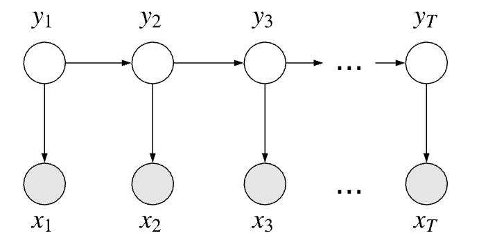
The hidden variables all share the Markov property that the the past is conditionally independent of the future given the present:
\[y_{t-1} \, \bot \, \{y_{t+1}, \dots ,y_{T}\} \mid y_t\]This property is also explicitly highlighted in the topology of the graph.
Furthermore, we can find how likely of the parse, given our HMM sequence, as followed:
The marginal and posterior distributions can be computed as follows:
- Marginal: $p(\mathbf{x}) = \sum\limits_{y_{1}}\cdots\sum\limits_{y_T} p(\mathbf{x,y})$
- Posterior: $p(\mathbf{y} \mid \mathbf{x}) = \frac{p(\mathbf{x,y})}{p(\mathbf{x})}$
Bayesian Network
- A BN is a directed graph whose nodes represent the random variables and whose edges represent directed influence of one variable on the another.
- It is a data structure that provides the skeleton for representing a joint distribution compactly in a factorized way.
- It offers a compact representation for a set of conditional independence assumptions about a distribution.
- We can view the graph as encoding a generative sampling process executed by nature, where
- the value for each variable is selected by the nature using a distribution that depends only on its parents. In other words, each variable is a stochastic function of its parents.
Bayesian Network: Factorization Theorem
We define $Pa_{X_i}$ and $NonDescendants_{X_i}$ as the set of parent nodes and not descendant nodes for the $i$th node, respectively. The topology of a directed graph asserts the set of conditional independence statements:
\[\{ X_i \, \bot \, NonDescendants_{X_i} \, | \, Pa_{X_i} \}\]
As a result, the joint probability of the above directed graph can be written as follows:
Specification of a Directed Graphical Model
There are two components to any GM:
- qualitative (topology)
- quantitative (numbers associated with each conditional distributions)
Sources of Qualitative Specifications
Where do our assumptions come from?
- Prior knowledge of causal relationship
- Prior knowledge of modular relationship
- Assessment from expert
- Learning from data
- We simply like a certain architecture (e.g. a layered graph)
- …
Local Structures & Independencies
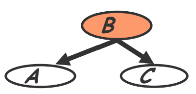
- Common parent (also called ‘common cause’ in section 3.3.1)
- Fixing $B$ decouples $A$ and $C$
- “Given the level of gene $B$, the levels of $A$ and $C$ are independent”
$A \perp C \mid B \Rightarrow P(A,C \mid B) = P(A \mid B) P(C \mid B)$Proof. We have the following: \begin{aligned} P(A,B,C) &= P(B)P(A \vert B)P(C \vert B) \\ P(A,C \vert B) &= P(A,B,C)/P(B) \end{aligned} Plugging in the above, $P(A,C \vert B)=P(B)P(A \vert B)P(C \vert B)/P(B)=P(A \vert B)P(C \vert B)$
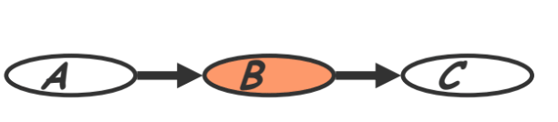
- Cascade (also called ‘causal/evidential trail’ in section 3.3.1)
- Knowing $B$ decouples $A$ and $C$
- “Given the level of gene $B$, the level gene $A$ provides no extra prediction value for the level of gene $C$”
- V-structure (also called ‘common effect’ in section 3.3.1)
- Knowing $C$ couples $A$ and $B$ because $A$ can “explain away” $B$ w.r.t. $C$
- “If $A$ correlates to $C$, then chance for $B$ to also correlate to $B$ will decrease”
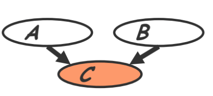
In class example of v-structure
My clock running late (event $A$) and a traffic jam (event $B$) which are independent events could both cause me to be late for class (event $C$). However, my presence couples the two events. Observe that if my clock was running late it could ‘explain away’ my lateness due to the traffic jam. In other words, $A$ and $B$ become coupled if $C$ is known because they jointly cause the 3rd event: $P(A,B)=P(A)P(B)$ but $P(A,B \vert C)$ cannot be decoupled into two conditionals.
I-maps
-
Definition (also see Definition 3.2-3.3): Let $P$ be a distribution over $X$. We define $I(P)$ to be the set of independence assertions of the form $(X \perp Y \vert Z)$ that hold in $P$.
-
Defn: Let $\mathcal{K}$ be any graph object associated with a set of independencies $I(K)$. We say that $\mathcal{K}$ is an I-map for a set of independencies $I$, if $I(\mathcal{K}) \subseteq I$.
-
We now say that $\mathcal{G}$ is an I-map for $\mathcal{P}$ if $\mathcal{G}$ is an I-map for $I(\mathcal{P})$, where we use $I(\mathcal{G})$ as the set of independencies associated.
Facts about I-map
-
For $\mathcal{G}$ to be an I-map of $\mathcal{P}$, it is necessary that $\mathcal{G}$ does not mislead us regarding independencies in $P$:
any independence that $\mathcal{G}$ asserts must also hold in $\mathcal{P}$. Conversely, $\mathcal{P}$ may have additional independencies that are not reflected in $\mathcal{G}$
This is formally defined in Definition 3.4.
In class examples
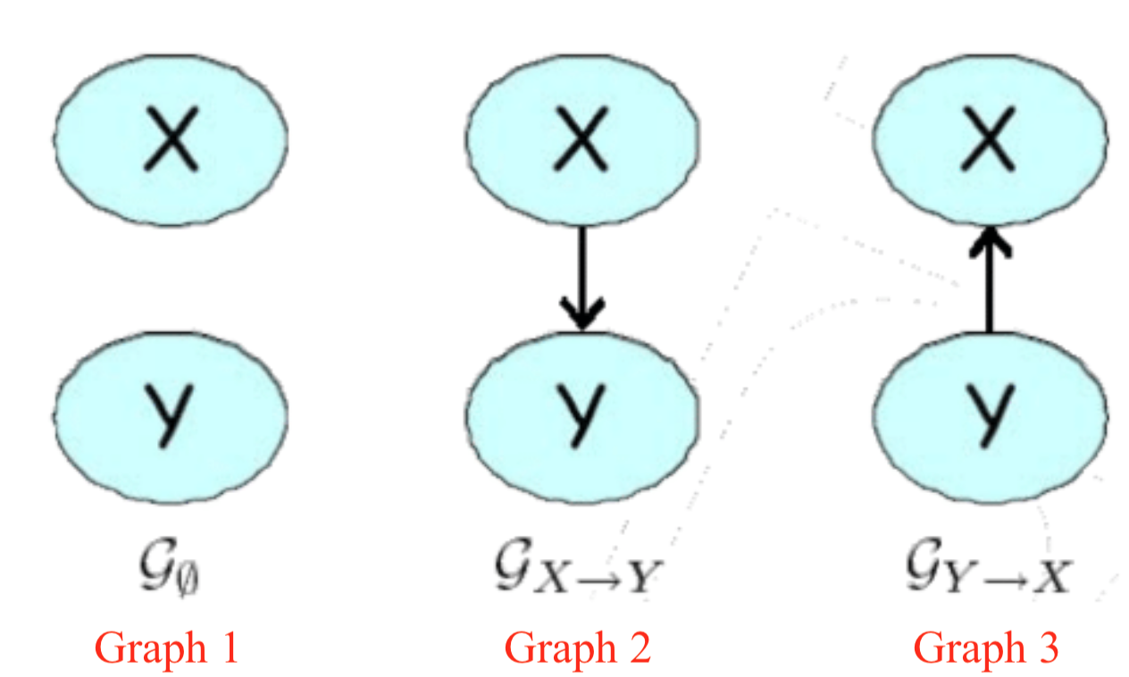
$X$ and $Y$ are independent only in Graph 1.
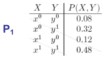
Below we have two tables showing the marginal distributions. Find the I-maps:
- $ P_1: I(P_1) = {X \perp Y} $ (from inspection i.e., $ P(X,Y)=P(X)P(Y), 0.48=0.6* 0.8 $)
Solution: Graph 1.
- $P_2: I(P_2) = \emptyset$
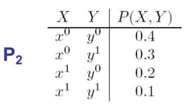
Solution: Both graph 2 and graph 3, since they assume no independences. Therefore, they are equivalent in terms of independent sets. Graph 1 has an independent set. Therefore it is not an I-map of $P_2$.
What is $I(G)$
Local Markov assumptions of BN
A Bayesian network structure $\mathcal{G}$ is a directed acyclic graph whose nodes represent random variables $X_1, \dots, X_n$ (also see the textbook definition 3.2.1).
Local Markov assumptions
Definition
Let \({Pa}_{X_i}\) denote the parents of \(X_i\) in \(\mathcal{G}\), and \(NonDescendants_{X_i}\) denote the variables in the graph that are not descendants of $X_i$. Then $\mathcal{G}$ encodes the following set of local conditional independence assumptions $I_{\ell}(\mathcal{G})$:
\[I_{\ell} (\mathcal{G}): \left\{ X_i \perp NonDescendants_{X_i} \vert Pa_{X_i}: \forall i \right\}\]In other words, each node $X_i$ is independent of its non-descendants given its parents.
D-separation criterion for Bayesian networks
Definition 1
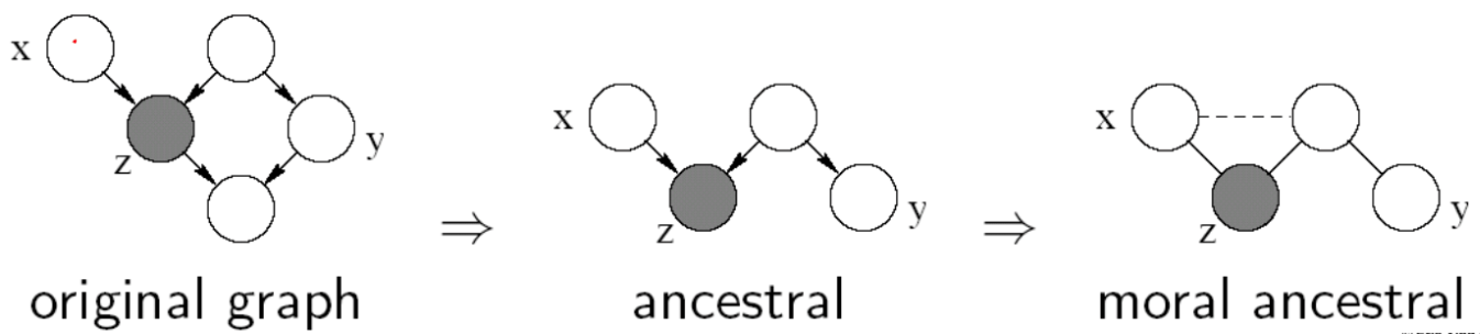
Variables $X$ and $Y$ are D-separated (conditionally independent) given $Z$ if they are separated in the moralized ancestral graph. (D stands for Directed edges.)
- Example: $ X \perp Y \vert Z$, then we say $Z$ D-separates $X$ and $Y$.
-
Ancestral graph (focusing only the nodes of interest): keeping only the nodes themselves + ancestors of the nodes in question.
-
Moral ancestral: remove the connectivity between nodes, but connect parents to nodes that are shared by a single child.
If there is a way to travel from one node to another node using any path (not through the given), then these two nodes are not conditionally independent (example is not conditionally independent).
Practical definition of $I(\mathcal{G})$
Global Markov properties of Bayesian networks
- $X$ is d-separated (directed-separated) from $Z$ given $Y$ if we can’t send a ball from any node in $X$ to any node in $Z$ using the “Bayes-ball” algorithm illustrated bellow (and plus some boundary conditions). Note this is expressed using math in Definition 3.7.
- Definition: $I(\mathcal{G}) =$ all independence properties that correspond to d-separation:
I(G) example
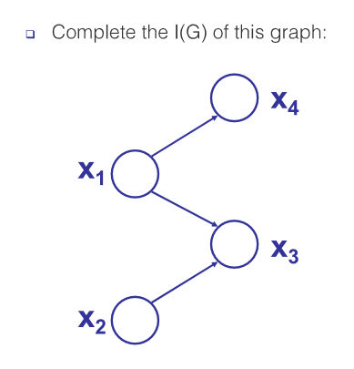
In this graph there are two types of active trail structures (see section 3.3.1 from the reading below for definition):
- common cause: $x_3 \leftarrow x_1 \rightarrow x_4$. This trail is active if we don’t condition on $x_1$.
- common effect: $x_2 \rightarrow x_3 \leftarrow x_1$. This trail is active if we condition on $x_3$.
To find the independencies, consider all trails with length greater than 1 (since a node cannot be independent of its parent).
Trails of length 2:
- $x_2 \rightleftharpoons x_3 \rightleftharpoons x_1$: due to ‘common effect’ structure, this trail is blocked as long as we do not condition on $x_3$. Therefore we get $(x_2 \perp x_1), (x_2 \perp x_1 \vert x_4)$.
- $x_3 \rightleftharpoons x_1 \rightleftharpoons x_4$: due to ‘common cause’ structure, this trail is blocked if we condition on $x_1$. Therefore we get \((x_3 \perp x_4 \vert x_1), (x_3 \perp x_4 \vert \{x_1, x_2\})\).
Trails of length 3 (only $x_2 \rightleftharpoons x_3 \rightleftharpoons x_1 \rightleftharpoons x_4$):
- due to ‘common effect’ structure $x_2 \rightarrow x_3 \leftarrow x_1$, this trail is blocked as long as we do not condition on $x_3$. Therefore we get $(x_2 \perp x_4), (x_2 \perp x_4 \vert x_1)$.
- due to ‘common cause’ structure $x_3 \leftarrow x_1 \rightarrow x_4$, this trail is blocked if we condition on $x_1$. Therefore we get \((x_2 \perp x_4 \vert x_1), (x_2 \perp x_4 \vert \{x_1, x_3\})\).
Trails between sets of nodes
- $x_2 \perp {x_1, x_4}$ : This is true by d-separation because we have seen that any path between $x_2$ and $x_1$, or between $x_2$ and $x_4$, is blocked.
Full $I(\mathcal{G})$
Putting the above together, and we have the following independencies.
The Equivalence Theorem
For a graph $G$, Let $D_1$ denotes the family of all distributions that satisfy $I(G)$. Let $D_2$ denotes the family of all distributions that factor according to $G$. Then $D_1 \equiv D_2$, which can be expressed as:
\[P(X)=\prod_{i=1:d}P(X_i \vert X_{\pi_i})\]This means separation properties in the graph imply independence properties about the associated variables.
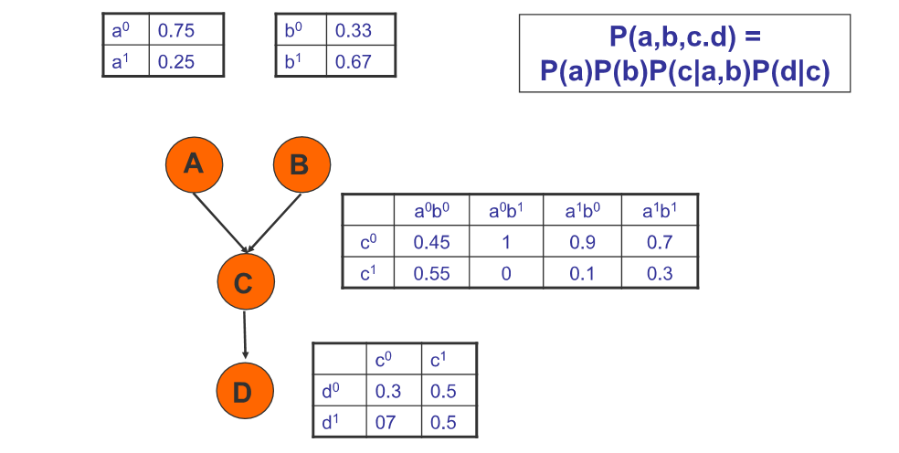
Conditional Probability Tables (CPTs)
This is an example with discrete probabilities.
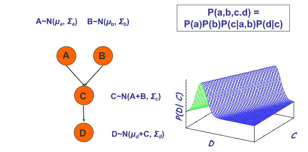
Conditional Probability Densities (CPDs)
The probabilities can also be a continuous function, e.g. the Gaussian distribution.
Summary of BN
-
Conditional independencies imply factorization.
-
Factorization according to $G$ implies the associated conditional independencies.
Soundness and Completeness of D-separation
Soundness and completeness are two desirable properties of d-separation, formally defined in Section 3.3.2
-
Soundness: If a distribution $P$ factorizes according to $G$, then $I(G) \subseteq I(P)$.
-
“Completeness”: (“Claim”) For any distribution $P$ that factorizes over $G$, if $(X \perp Y \vert Z) \in I(P)$, then $\text{d-sep}_{\mathcal{G}} (X; Y \vert Z)$)
-
Actually, the “Completeness” is not holding true all the time. “Even if a distribution factorizes over \(G\), it can still contain additional independencies that are not reflected in the structure.”
Example (follows Example 3.3 from textbook):
Consider a distribution $P$ over two independent variables $A$ and $B$. Recall that every independence we can observe from an I-map is by definition encoded in $P$ (see Definition 3.2-3.3 from the readings below). One I-map for $P$ would be the DAG $A \rightarrow B$ since it encodes no independencies. This is because $\varnothing$ is a subset of every set.
However, we can manipulate the conditional probability table so that independencies hold in \(P\) which do not follow from D-separation. One such conditional probability table would be:
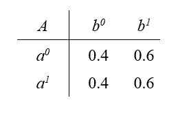
Observe that in this table, $B$ is independent of $A$. But this is not reflected in the I-map $A \rightarrow B$.
Theorem
Let $G$ be a BN graph. If $X$ and $Y$ are not d-separated given $Z$ in $G$, then $X$ and $Y$ are dependent in some distribution $P$ that factorizes over $G$.
Theorem:
For almost all distributions $P$ that factorize over $G$, i.e., for all distributions except for a set of “measure zero” in the space of CPD parameterizations, we have that $I(P)=I(G)$.
Readings
The Bayesian network representation
3.1.1 Exploiting independence Properties
Standard vs compact parametrization of independent random variables
Given random variables $X_i$ each representing the outcome of an independent coin toss, the standard parametrization of their joint distribution would be as follows:
Note there are 2 possibilities for each outcome $x_i$, this representation requires $2^n$ parameters. However, only $2^n -1$ will be independent parameters since the last probability is fully determined by the first $2^n$ (all probabilities sum to 1).
One simple way to reduce the number of parameters needed, would be to represent the probability that each coin toss lands heads as $ \theta_1, … \theta_n $. Then we have the following compact representation requiring only $n$ parameters:
\[P(X_1, ... X_n) = \prod_i \theta_{X_i}\]3.1.3 Naive Bayes
We can further express the joint distribution in terms of conditional probabilities. This is done in the Naive Bayes model.
Instances of this model will include:
- class: some category $ C \in {c^1, …c^k} $ which gives a prior on the value of each feature
- features: observed properties $X_1, … X_k$
The model makes the strong ‘naive’ conditional independence assumption:
\[P(x_i | C, x_1, \dots, x_n) = P(x_i | C)\]In words, features are conditionally independent, given the class of the instance of this model. Thus the joint distribution of the Naive Bayes model factorizes as follows: \(P(C, X_1, ... X_n) = P(C) \prod_i P(X_i |C)\)
3.2.1 Bayesian networks
Bayesian networks use a graph whose nodes are the random variables in the domain, and whose edges represent conditional probability statements. Unlike in the Naive Bayes model, Bayesian networks can also represent distributions that do not satisfy the naive conditional independence assumption.
Definition 3.1: Bayesian Network (BN)
A bayesian network $\mathcal{G}$ is a directed acyclic graph, whose nodes represent random variables $X_1, …X_n $. Let $Pa_{X_i}^{\mathcal{G}}$ denote the parents of $X_i \in \mathcal{G}$ and $NonDescendants_{X_i}$ denote the variables in the graph which are not descendants of $X_i$. Then $\mathcal{G}$ encodes the following set of conditional independence assumptions, also called the ‘local independencies’ and denoted by $I_l(\mathcal{G})$:
For each variable $X_i: (X_i \perp NonDescendants_{X_i} \vert \text{Pa}_{X_i}^{\mathcal{G}})$
3.2.3 Graphs and Distributions
In this section it is shown that the distribution $P$ satisfies the local independencies associated with $\mathcal{G} \iff P$ is representable as a set of conditional probability distributions (CPDs) associated with $\mathcal{G}$.
Definition 3.2-3.3: I-Map
Let $P$ be a distribution over $\mathcal{X}$. We define $I(P)$ to be the set of independence assertions of the form $X \perp Y \vert Z$ that hold in $P$.
Let $\mathcal{K}$ be any graph object associated with a set of independencies $I(\mathcal{K})$. We say $\mathcal{K}$ is an I-map for $I$ if $I(\mathcal{K}) \subseteq I$.
Note this means that $\mathcal{G}$ is an I-map for $P $ if $\mathcal{G}$ is an I-map for $I(P)$.
I-Map to factorization
In this section it is proven (see text) that the conditional independence assumptions implied by the BN structure $\mathcal{G}$ allow us to factorize the distribution $P$ for which $\mathcal{G}$ is an I-map into conditional probability distributions.
Definition 3.4 Factorization
Let $P$ be a distribution and $\mathcal{G}$ be a BN graph over random variables $X_1, …X_n $. We say that $P$ factorizes according to $\mathcal{G}$ if $P$ can be expressed as a product:
\[P(X_1, ... X_n) = \prod_i P( X_i | \text{Pa}_{X_i}^{\mathcal{G}})\]Reduction in number of parameters
In a distribution over $n$ binary variables, specifying the joint distribution will require $2^n - 1$ independent parameters (as stated in 3.1.1). However if the distribution factorizes according to $\mathcal{G}$ where each node has at most $k$ parents, then the number of independent parameters is $ < 2^k$. Since $k$ is usually small, this represents an exponential reduction in number of parameters.
Factorization to I-map
The converse also holds as given by the following :
Theorem 3.2
Let $\mathcal{G}$ be a BN graph over random variables $X $ and $P$ be a distribution over the same space. If $P$ factorizes according to $\mathcal{G}$ then $\mathcal{G}$ is an I-map for $P$.
Box 3.C Knowledge engineering
Building a BN in the real world requires many steps including:
- picking variables precisely: we need some variables that can be observed, and their domain should be specified. Sometimes introducing hidden variables will help to render the observed variables conditionally independent.
- picking a structure consistent with the causal order: choose enough variables to approximate the causal relationships.
- picking probability estimates for events in the network: data collection may be difficult but small errors have little effect (though the network is sensitive to events assigned a zero probability, and to relative size of probabilities of events)
Done correctly, the model will be useful as well as not too complex to use (see Box 3.D).
3.3.1 D-separation
Objective: determine which independencies hold for every distribution $P$ which factorizes over $G$.
Definition 2.16 Trail
We say that $X_1, … X_k$ form a trail in the graph $\mathcal{K} = (\mathcal{X}, \mathcal{E}) $ if for every $i = 1, … , k-1$ we have that $ X_i \rightleftharpoons X_{i+1}$.
Types of active two edge trails
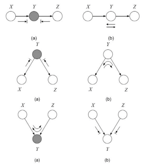
By examining 2-edge connections between nodes $X,Y,Z$ four types of active trails, i.e. trails along which influence can flow from $X$ to $Z$, are apparent:
- Causal trail $X \rightarrow Z \rightarrow Y$ : active iff Z is not observed.
- Evidential trail $X \leftarrow Z \leftarrow Y$ : active iff Z is not observed.
- Common cause $X \leftarrow Z \rightarrow Y$ : active iff Z is not observed.
- Common effect $X \rightarrow Z \leftarrow Y$ : active iff Z or one of its descendants is observed.
For influence to flow through a longer trail $ X_1 \rightleftharpoons … \rightleftharpoons X_n $, every two-edge trail within must allow influence flow. This is summarized as follows:
Definition 3.6 active trail
Let $\mathcal{G}$ be a BN structure and. $ X_1 \rightleftharpoons … \rightleftharpoons X_n $ be a trail in $\mathcal{G}$. Let $Z$ be a subset of observed variables. Then the trail $ X_1 \rightleftharpoons … \rightleftharpoons X_n$ is active given $Z $ if:
- Whenever we have a v-structure $ X_{I-1} \to X_i \leftarrow X_{I+1} $ then $X_i$ or one of its descendants are in $Z$
- No other node along the trail is in $Z$
Further, for directed graphs that may have more than one trail between nodes “directed separation” (d-separation) gives a notion of separation between nodes.
Definition 3.7 D-separation
Let $X,Y,Z$ be three sets of nodes in $\mathcal{G}$. We say that $X, Y$ are d-separated given $Z$ (denoted $ \text{d-sep}_{\mathcal{G}} (X; Y \vert Z) $ ) if there is no active trail between any node X $ \in X $ and Y $ \in Y $ given $Z$.
3.3.2 Soundness and Completeness
As a method d-separation has the following properties (proof in text):
Soundness: $ X, Y $ are d-separated given $ Z \implies X \perp Y \vert Z $ i.e. independence determined by d-separation is satisfied by the underlying distribution.
Completeness: If $ X \perp Y \vert Z $ then they are d-separated, i.e. d-separation detects all possible independencies.