Lecture 3: Undirected Graphical Models

An introduction to undirected graphical models

Review

In addition to the I-map concept that was introduced in the last lecture, today’s lecture also includes minimal I-map.

Minimal I-maps

A DAG $\mathcal{G}$ is a minimal I-map if it is an I-map for a distribution $P$, and if the removal of even a single edge from $\mathcal{G}$ renders it not an I-map.

A distribution may have several minimal I-maps, each corresponding to a specific node-ordering.
The fact that $\mathcal{G}$ is a minimal I-map for $P$ is far from a guarantee that $\mathcal{G}$ captures the independence structure in $P$.

“Bayes-ball” Algorithm

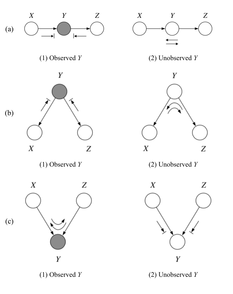
“Bayes-ball” algorithm is an algorithm that we can apply to retrieve independences directly from a graphical model. We say $X$ is d-separated from $Z$ given $Y$ if we cannot send a ball from any node in $X$ to any node in $Z$. The conditional probability statement (“given $Y$”) is represented by shading the node in the graph. Examples of three basic directed graphical structures are shown below.

In (a) and (b), the shaded $Y$ node blocks the ball from going between nodes $X$ and $Z$. This gives the independence relation that was introduced in the last lecture: $X \perp Z \mid Y$.
(c), also called the “V-structure”, is a special case. Opposite from the first two exmaples, the ball can go between $X$ and $Z$ if the node $Y$ is shaded, and is blocked otherwise. Therefore, the graph on the right yields $X \perp Z$.

With these basic structures, we can apply the rules on a DAG. For example, let us try to find whether $X_2$ and $X_3$ are independent given $X_1$ and $X_6$.

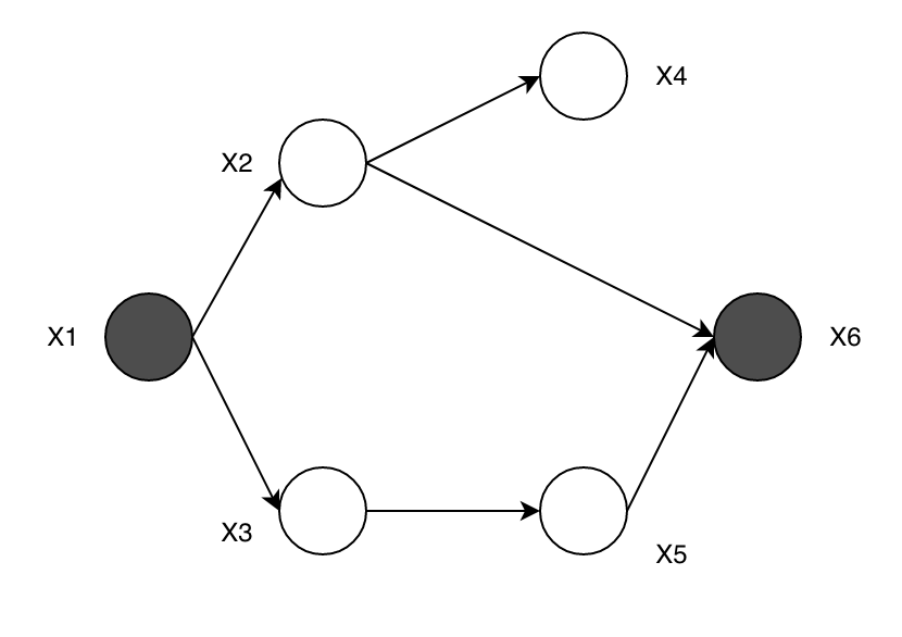
After shading $X_1$ and $X_6$, the ball cannot go from $X_2$ to $X_3$ through $X_1$ because it is blocked; however, $X_2$, $X_6$, and $X_5$ forms a “V-structure”, so the ball can go along the path $X_2$, $X_6$, $X_5$, $X_3$. Therefore, the independence statement is invalid.

Limits of Directed and Undirected GMs

From a representational perspective, we aim to find a graph $\mathcal{G}$ that precisely captures the independencies in a given distribution $P$. This goal of learning GMs motivates the following definition.

Perfect Maps

We say that a graph $\mathcal{G}$ is a perfect map (P-map) for a set of independencies $\mathcal{I}$ if $\mathcal{I}(\mathcal{G}) = \mathcal{I}$. We say that $\mathcal{G}$ is a perfect map for $P$ if $\mathcal{I}(\mathcal{G}) = \mathcal{I}(P)$. That is, $\text{sep}_{\mathcal{G}}(X;Z \vert Y) \iff P \models (X \perp Z \vert Y)$.

The P-map of a distribution is unique up to I-equivalence between networks. That is, a distribution P can have many P-maps, but all of them are I-equivalent.

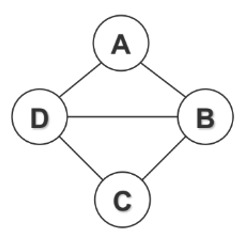
Arbitrary distribution $P$’s, however, do not necessarily attain perfect maps as either undirected or directed GMs. Two such examples are shown below.

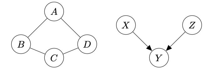
**A Venn diagram illustration of graphical model families, where D is the family of directed GMs, and U the family of undirected GMs.**

Left: A distribution with no possible DGM representation, which entails $A\perp C\vert \{B,D\}$ and $B\perp D\vert \{A,C\}$. Right: The v-structure is a distribution with no UGM representation.

Undirected Graphical Models - Overview

There can only be symmetric relationships between a pair of nodes (random variables). In other words, there is no causal effect from one random variable to another.
The model can represent properties and configurations of a distribution, but it cannot generate samples explicitly.
Each node has strong correlations with its neighbors.

Example

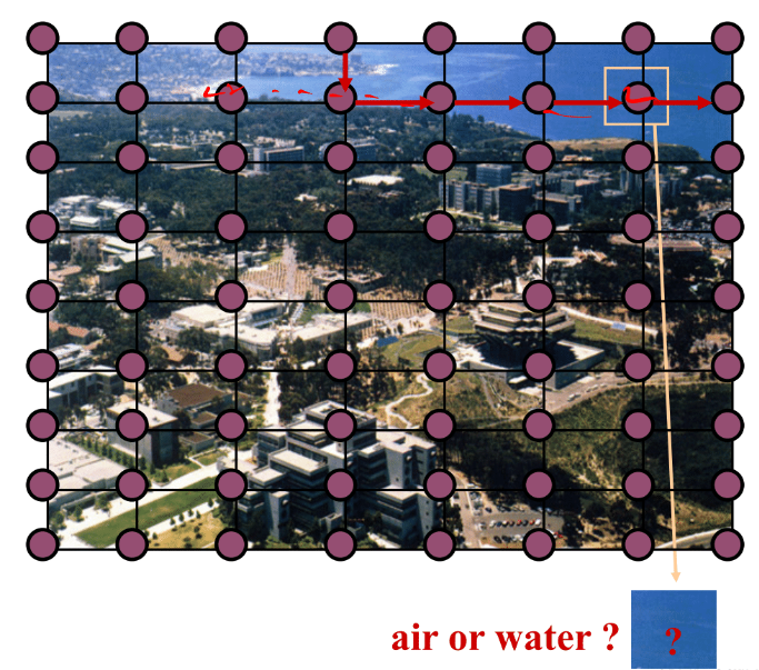
Let each node represents an image patch. It is impossible to tell what is inside this image patch by isolating it from others. However, when we look at its neighboring image patches, we can see that it’s an image patch of water. Due to the fact that the relationships between neighboring image patches should be symmetric, an image is best represented by an undirected graphical model. This particular undirected graphical model is also known as the grid model.

Quantitative Specification

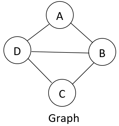
Cliques

Cliques are subgraphs that are fully connected.
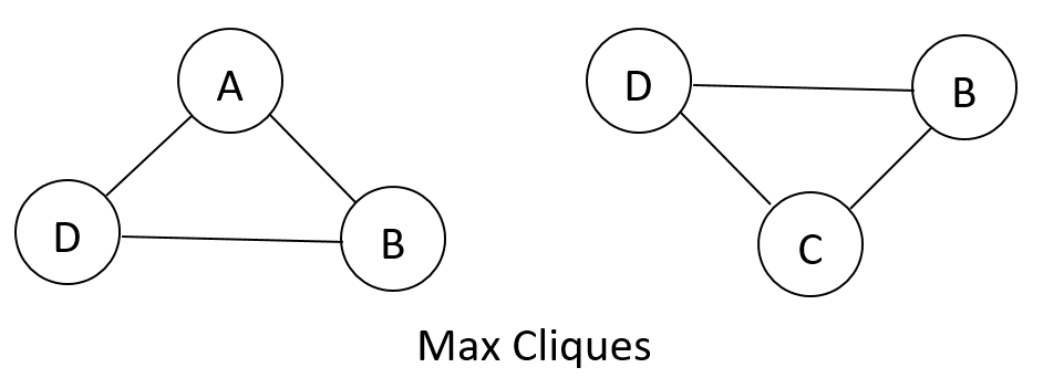
A maximal clique is a clique such that any superset (any bigger subgraph that contains this subgraph) is not a complete graph.
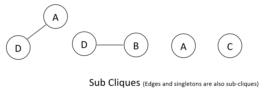
A sub-clique is a not-necessarily-maximal clique.
Example

Potential Functions

Each clique can be associated with a potential function $\psi$, which can be understood as a provisional function of its arguments that assigns a pre-probabilistic score of their joint distribution. This potential function can be somewhat arbitrary, but must be non-negative.

Why cliques? Each component of the clique contributes to the overall potential function.

Example

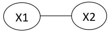
For $\psi_c(X_1, X_2)$,

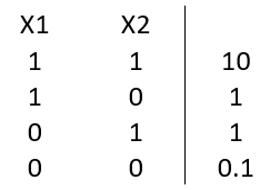
**This table represents the potential function values given combinations of random variable inputs.**

Potential functions are not necessarily probabilistic:

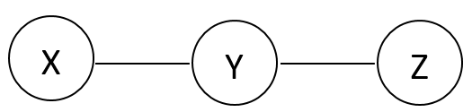
**Another example used to illustrate potential functions.**

This model implies that $X \perp Z | Y$. This independence statement implies (by definition) that the joint must factorize as:

\begin{aligned} p(x,y,z)&=p(y)p(x|y)p(z|y) \\ &=p(x,y)p(z|y) \\ &=p(x|y)p(y,z) \end{aligned}

Probability distributions can be used as potential functions. However, in this case, we cannot let all potentials be either marginal probabilities or conditional probabilities. So the potential function for this graph cannot be probability distributions.

Gibbs Distribution and Undirected Graphical Model Definition

Given an undirected graph $H$ and clique potentials functions $\psi_C$ associated with cliques of $H$, we say $P(X_1, ..., X_n)$ is a Gibbs distribution over $H$ if it can be represented as

\[P(X_1, ..., X_n)=\frac{1}{Z}\prod_{c\in C}{\psi_c(\bold{x_c})}\]

where $Z$ is also known as the partition function. Upper case $C$ denotes the set of all cliques, and lower case $c$ denotes a clique associated with a set of random variables $\bold{x}$.

An undirected graphical model represents a distribution $P(X_1, ..., X_n)$ defined by an undirected graph $H$, a set of positive potential functions $\psi_C$ and the associated cliques of $H$, such that

\begin{aligned} P(X_1,...,X_n)=\frac{1}{Z}\prod_{c\in C}{\psi_c(\bold{x_c})} \\ Z=\sum_{x_1,...,x_n}\prod_{c\in C}{\psi_c(\bold{x_c})} \end{aligned}

Note that this distribution is the Gibbs distribution.

Example UGM Models Depending on the question of interest, different representations may be more appropriate.

**An example graph used to illustrate UGM.**

Using Max Cliques

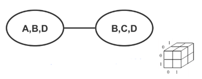
\begin{aligned} P'(A,B,C,D)=\frac{1}{Z}\psi_c(A,B,D)\psi_c(B,C,D) \\ Z=\sum_{A,B,C,D}\psi_c(A,B,D)\psi_c(B,C,D) \end{aligned}

We only need to represent discrete nodes with two 3D tables instead of one 4D table.

Using Pairwise Cliques

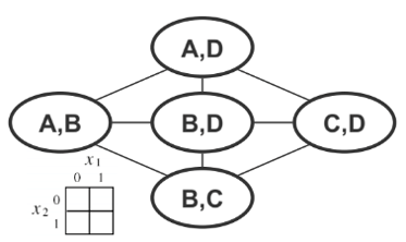
\begin{aligned} P''(A,B,C,D)=\frac{1}{Z}\psi_c(A,B)\psi_c(A,D)\psi_c(B,C)\psi_c(B,D)\psi_c(C,D) \\ Z=\sum_{A,B,C,D}\psi_c(A,B)\psi_c(A,D)\psi_c(B,C)\psi_c(B,D)\psi_c(C,D) \end{aligned}

We only need to represent discrete nodes with five 2D tables instead of one 4D table.

Using Canonical Representation

Even if we use fine-grained representation, the Markov network is often overparameterized. For any given distribution, there are multiple choices of parameters to describe in the model. As shown above, we can either choose max cliques or pairwise cliques to represent this model. Furthermore, ambiguities can arise in clique structures. For example, given a pair of cliques $\{A, B\}$ and $\{B, C\}$, the information about $B$ can be placed in either of the two cliques, resulting in many ways to specify the samme distribution.

The canonical representation provides a natural approach to avoid this problem. It is defined over all non-empty cliques as shown below.Please refer to Koller and Friedman Texbook Ch.4, page 129 for details. The formula performs an inclusion-exclusion computation to make sure that each random variable contributes exactly once to the overall function.

\begin{aligned} P'''(A,B,C,D)&=\frac{1}{Z}\psi_c(A,B,D)\psi_c(B,C,D) \\ & \times\psi_c(A,B)\psi_c(A,D)\psi_c(B,C)\psi_c(B,D)\psi_c(C,D) \\ & \times\psi_c(A)\psi_c(B)\psi_c(C)\psi_c(D) \end{aligned}

\begin{aligned} Z&=\sum_{A,B,C,D}\psi_c(A,B,D)\psi_c(B,C,D) \\ & \times\psi_c(A,B)\psi_c(A,D)\psi_c(B,C)\psi_c(B,D)\psi_c(C,D) \\ & \times\psi_c(A)\psi_c(B)\psi_c(C)\psi_c(D) \end{aligned}

Qualitative Specification

Global Markov Independency

Suppose we are given the following UGM, denoted by $H$:

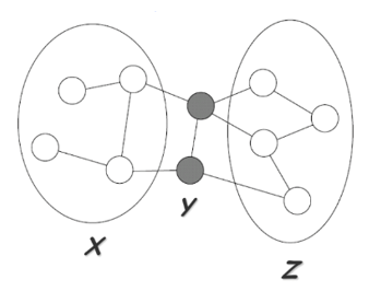
$Y$ separates $X$ and $Z$ if every path from a node in $X$ to a node in $Z$ passes through a node in $Y$:

\[sep_H(X;Z|Y)\]

A probability distribution satisfies the global Markov property if for any disjoint X,Y,Z such that Y separates X and Z, X is independent of Z given Y.

\[\mathcal{I}(H)=\{X\perp Z | Y:sep_H(X;Z|Y)\}\]

Local Markov Independency

For each node $X_i\in \bold{V}$, there is a unique Markov blanket of $X_i$, denoted $MB_{X_i}$, which is the set of neighbors of $X_i$ in the graph.

The local Markov independencies ($\mathcal{I}_l$) associated with $H$ is:

\[\mathcal{I}_l(H):\{X_i \perp (\bold{V}-\{X_i\}-MB_{X_i})|MB_{X_i}:\forall i\}\]

In other words, $X_i$ is independent of the rest of the nodes given its immediate neighbors $MB_{X_i}$.

Soundness and Completeness of Global Markov Property

The global Markov property for UGMs is similar to its variant for DGMs, in the sense that they both attain similar soundness and completeness results.

Soundness

Theorem: Let $P$ be a distribution over $\mathcal{X}$, and $\mathcal{G}$ a Markov network structure over $\mathcal{X}$. If $P$ is a Gibbs distribution that factorizes over $\mathcal{G}$, then $\mathcal{G}$ is an I-map for $P$.

Proof: Let $X,Y,Z$ be three disjoint subsets in $\mathcal{X}$ such that $Z$ separates $X$ and $Y$ in $\mathcal{G}$. We will show that $P\models (X\perp Y\vert Z)$.

First, we observe that there is no direct edge from $X$ to $Y$. Assuming that $(X,Y,Z)$ is a partition of $\mathcal{X}$, we know that any clique in $\mathcal{G}$ is fully attained in either $X\cup Z$ or $Y\cup Z$. Let $\mathcal{I}_{X}$ be the indices of the set of cliques that are contained in $X\cup Z$, and $\mathcal{I}_{Y}$ be the set defined for $Y\cup Z$. We know that

\[P(X_1,\cdots,X_n) = \frac{1}{Z}\prod_{i\in \mathcal{I}_X}\phi_i (D_i)\cdot \prod_{i\in \mathcal{I}_Y}\phi_i (D_i).\]

None of the terms in the first product contains variable from the latter. Hence, we can rewrite this product in the form:

\[P(X_1,\cdots,X_n) = \frac{1}{Z}f(X,Z)g(Y,Z),\]

and we observe that independence follows.

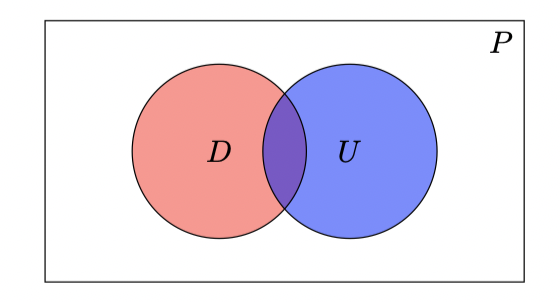
If $X\cup Y\cup Z$ is a strict subset of $\mathcal{X}$. Let $U = \mathcal{X}\setminus (X\cup Y\cup Z)$. We can partition $U$ into two disjoint sets $U_1$ and $U_2$ such that $Z$ separates $X\cup U_1$ from $Y\cup U_2$ in $\mathcal{G}$. Using our argument from the partition case, we have that $\big((X\cup U_1)\perp ((Y\cup U_2)\vert Z$. Apply decomposition property of probability we attain that $P\models (X\perp Y\vert Z)$. $\square$

Completeness (Hammersley-Clifford theorem)

Theorem: Let $P$ be a positive distribution over $\mathcal{X}$, and $\mathcal{G}$ a Markov network graph over $\mathcal{X}$. If $\mathcal{G}$ is an I-map for $P$, then $P$ is a Gibbs distribution that factorizes over $\mathcal{G}$.

This result shows that, for positive distributions, the global independencies imply that the distribution factorizes according to the network structure. Thus, for this class of distributions, we have that a distribution $P$ factorizes over a Markov network $\mathcal{G}$ if and only if $\mathcal{G}$ is an I-map for $P$.

Other Markov Properties

For UGMs, we defined I-maps in terms of global Markov properties. We will now define local independence. Intuitively, when two variables are not directly linked, there must be some way of rendering them conditionally independent. Specifically, we can require that $X$ and $Y$ be independent given all other nodes in the graph.

Pairwise Independencies

Let $\mathcal{G}$ be a Markov network. We define the pairwise independencies associated with $\mathcal{G}$ to be

\[\mathcal{I}_P(\mathcal{G}) = \{(X\perp Y\vert \mathcal{X}-\{X,Y\}): X-Y\notin \mathcal{G}\}\]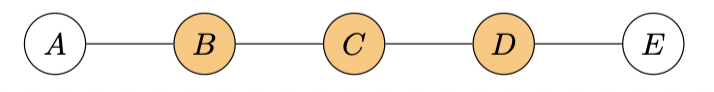

To illustrate this idea, observe that in the figure above, the variables of interests, $A$ and $E$, are conditionally independent given all other nodes in the graph, $\{B,C,D\}$.

Pairwise and local indepdencies are also related. Their relationships are described in the following propositions and theorem.

Proposition

1. For any Markov network $\mathcal{G}$ and any distribution $P$, we have that if $P\models \mathcal{I}_l(\mathcal{G})$ then $P\models \mathcal{I}_P(\mathcal{G})$.

2. For any Markov network $\mathcal{G}$ and any distribution $P$, we have that if $P\models \mathcal{I}(\mathcal{G})$ then $P\models \mathcal{I}_l(\mathcal{G})$.

3. Let $P$ be a positive distribution. If $P$ satisfies $\mathcal{I}_P(\mathcal{G})$, then $P$ satisfies $\mathcal{I}(\mathcal{G})$.

Theorem

The followings are equivalent for a positive distribution $P$:

$P\models \mathcal{I}_l(\mathcal{G})$

$P\models \mathcal{I}_P(\mathcal{G})$

$P\models \mathcal{I}(\mathcal{G})$

Exponential Form

Since we don’t want to constraint the clique potentials to be positive in all situations, exponential form is used to represent a clique potential $\phi_c(x_c)$ in an unconstrained form using a real-value “energy” funtion $\phi_c(x_c)$:

\[\Phi_c(x_c)=\exp\bigg\{-\phi_c(x_c)\bigg\}\]

This then gives the joint probability a nice additive structure

\[p(x)=\frac{1}{Z}\exp\bigg\{-\sum_{c\in C}\phi_c(x_c)\bigg\}=\frac{1}{Z}\exp\bigg\{-H(x)\bigg\}\]

where the sum in the exponent is called the “free energy”:

\[H(x) = \sum_{c\in C}\phi_c(x_c)\]

This form of representation is called the “Boltzmann distribution” in physics, and a log-linear model in statstics.

Undirected Graph Exmples

In this section, we cover several well-known undirected graphical models: Boltzmann Machine (BM), Ising model, Restricted Boltzmann Machine (RBM), and Conditional Random Field (CRF).

Boltzmann Machine (BM)

Boltzmann Machine is a fully connected graph with pairwise (edge) potentials on binary-valued nodes. One example is shown in the following figure:

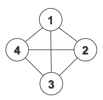
Its probability distribution can be written as:

\[p(x_1,x_2,x_3,x_4)=\frac{1}{Z}\exp\bigg\{\sum_{ij}\phi_{ij}(x_i,x_j)\bigg\}\]

It could also be written in a quadratic way:

\[p(x_1,x_2,x_3,x_4)=\frac{1}{Z}\exp\bigg\{\sum_{ij}\theta_{ij}x_ix_j+\sum_i\alpha_ix_i+C\bigg\}\]

Hence the overall free energy function has the form:

\[H(x)=\sum_{ij}(x_i-\mu)\Theta_{ij}(x_j-\mu)=(x-\mu)^T\Theta(x-\mu)\]

which can then be solved using quadratic programming.

Ising model

In the Ising model, nodes are arranged in a regular topology (often a regular packing grid) and connected only to their geometric neighbors. It is like a sparse Boltzmann Machine. There is also the multi-state Ising model (also called Potts model), in which nodes can take multiple values instead of just binary values. One example of Ising model is shown in the following figure:

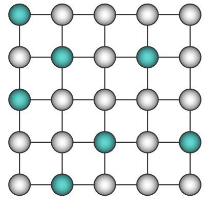
Its probability distribution can be written as

\[p(X)=\frac{1}{Z}\exp\bigg\{\sum_{i,j\in N_i}\theta_{ij}X_iX_j+\sum_i \theta_{i0}X_i\bigg\}\]

Restricted Boltzmann Machine (RBM)

The Restricted Bolzmann Machine is a bipartite graph with connections between one layer of hidden units and one layer of visible units. One example is shown in the following figure:

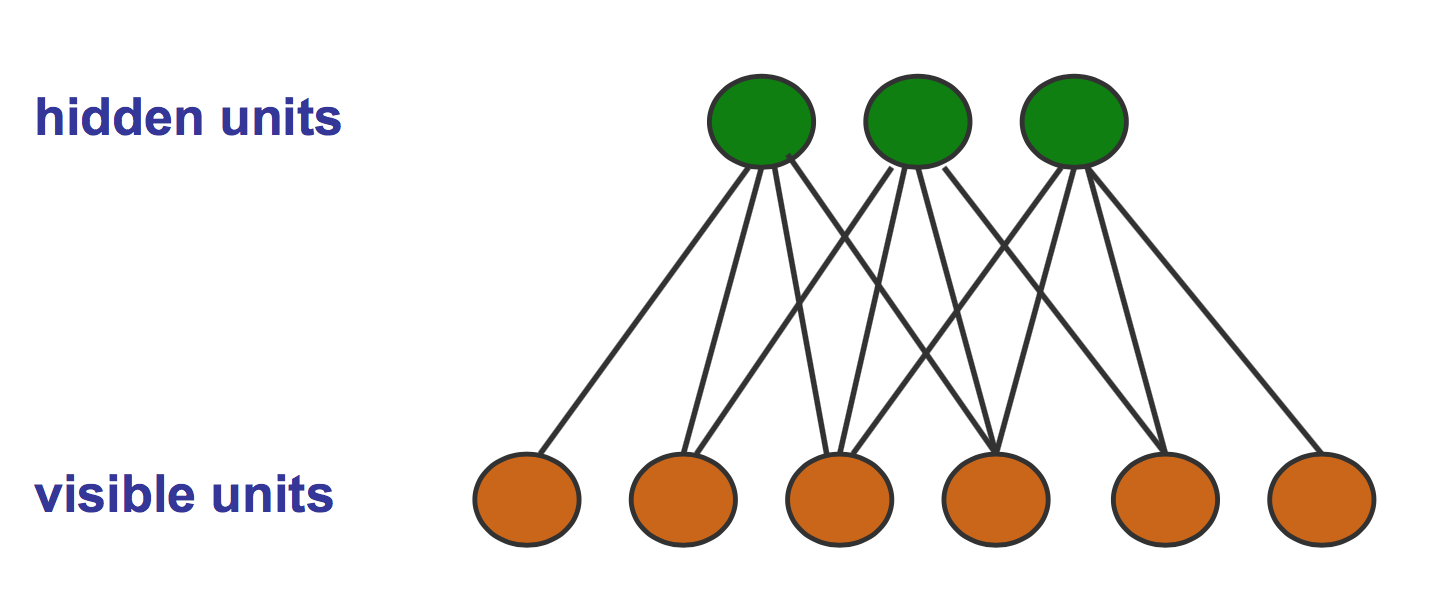
Its probability distribution can be written as

\[p(x,h|\theta)=\exp\bigg\{\sum_i\theta_i\phi_i(x_i) + \sum_j\theta_j\phi_j(h_j) + \sum_{i,j}\theta_{i,j}\phi_{i,j}(x_i,h_j)-A(\theta)\bigg\}\]

RBM has some appealing properties. For example, factors are marginally dependent and factors are conditionally independent given observations on the visible nodes. They enable one to use iterative Gibbs sampling for inference and learning on RBM. If the edges in RBM were directed, there would be plenty of V-structures in the graph (lots of dependences) that increase the inference difficulty.

Conditional Random Field (CRF)

Conditional random field is an analogous form of HMM in the undirected case. It allows arbitrary dependencies on the input. For example, when labeling $X_i$, future observations can be taken into account. An example of CRF is shown in the figure:

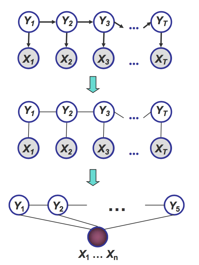
The probability distribution could be written as

\[p_\theta(y|x)=\frac{1}{Z(\theta,x)}\exp\bigg\{\sum_c\theta_cf_c(x,y_c)\bigg\}\]

Lecture 3: Undirected Graphical Models

Review

Minimal I-maps

“Bayes-ball” Algorithm

Limits of Directed and Undirected GMs

Perfect Maps

Undirected Graphical Models - Overview

Example

Quantitative Specification

Cliques

Example

Potential Functions

Example

Gibbs Distribution and Undirected Graphical Model Definition

Example UGM Models Depending on the question of interest, different representations may be more appropriate.

Using Max Cliques

Using Pairwise Cliques

Using Canonical Representation

Qualitative Specification

Global Markov Independency

Local Markov Independency

Soundness and Completeness of Global Markov Property

Soundness

Completeness (Hammersley-Clifford theorem)

Other Markov Properties

Pairwise Independencies

Proposition

Theorem

\(P\models \mathcal{I}_l(\mathcal{G})\)

\(P\models \mathcal{I}_P(\mathcal{G})\)

\(P\models \mathcal{I}(\mathcal{G})\)

Exponential Form

Undirected Graph Exmples

Boltzmann Machine (BM)

Ising model

Restricted Boltzmann Machine (RBM)

Conditional Random Field (CRF)