Lecture 5: Parameter Estimation in Fully Observed Bayesian Networks

Introduction to the problem of Parameter Estimation in fully observed Bayesian Networks

Introduction

Last class, we presented two major types of graphical model task, Inference and Learning, and we mainly discussed about inference. In this lecture, we start to introduce the learning task, and explore some learning techniques used in fully observable Bayesian Networks.

Learning Graphical Models

Before we get started, it’s better for us to get some intuition about what learning is and which goal learning is achieving.

The goal

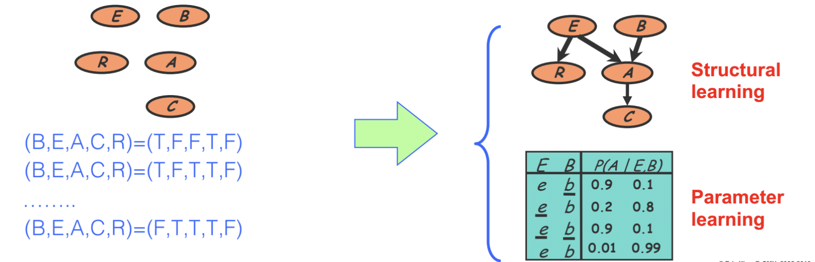
The goal: Given a set of independent samples (assignments of random variables), find the best (or the most likely) Bayesian Network (both DAG and CPDs).

As shown in the figure below, we are given a set of independent samples (assignments of binary random variables). Assume it’s a DAG, we are going to learn the directed links (causality relationships) between nodes, this process is called Structural Learning. Learning the conditional possibility is another task called Parameter learning.

Overview

As listed below, there’re several learning scenarios we are interested in:

Completely observed GMs:
- 1.1. directed
- 1.2. undirected
Partially or unobserved GMs:
- 1.1. directed
- 1.2. undirected (an open research topic)

Some useful estimation principles are also listed here:

Maximal likelihood estimation (MLE)
Bayesian estimation
Maximal conditional likelihood
Maximal “Margin”
Maximum entropy

We use learning as a name for the process of estimating the parameters, and in some cases, the topology of the network, from data.

Parameter Learning

In this section, we are going to introduce Parameter Learning, and some useful related models.

When doing parameter learning, we assume that the Graphical model G itself is known and fixed, G could come from either expert design or an intermediate outcome of iterative structure learning.

The goal of parameter learning is to estimate parameters from a dataset of $N$ independent, identically distributed (i.i.d.) training samples $D = {x_1, \cdots, x_N}$.

In general, each training case $\mathbf{x}_n = (x_{n,1}, \cdots, x_{n, M})$ is a vector of $M$ values, one per node. Depending on the model, elements in $\mathbf{x}_n$ could be all known (no missing values, no hidden variables) if the model is completely observable, or partially known ($\exists i, x_{n,i}$ is not observed) if the model is partially observable.

In this class, we mainly consider learning parameters for a BN that is completely observable with a given structure.

Exponential Family Distributions

There are various density estimation tasks that can be viewed as single-node GMs (see the supplementary section for examples), and they are in fact instances of Exponential Family Distributions.

Exponential Family Distributions are building blocks for general GMs, and have nice properties allowing us to easily do MLE and Bayesian estimation.

Definition

For a numeric random variable $X$,

\[p_X(x|\eta) = h(x)\exp\{\eta^T T(x) - A(\eta)\}=\frac{1}{Z(\eta)}h(x)\exp\{\eta^T T(x)\}\]

Function $T(x)$ is a sufficient statistic (will be explained in sufficiency section).

Function $A(\eta) = \log{Z(\eta)}$ is the log normalizer.

Examples

We can see lots of probability distributions actually belonging to this family (including Bernoulli, Multinomial, Gaussian, Poisson, Gamma).

Example 1: Multivariate Gaussian Distribution

For a continuous vector random variable $X \in R^k$:

\begin{aligned} p_X(x|\mu,\Sigma) &= \frac{1}{(2\pi)^{k/2}|\Sigma|^{1/2}}\exp\left\{-\frac{1}{2}(x-\mu)^T \Sigma^{-1}(x-\mu)\right\} \\ &= \frac{1}{(2\pi)^{k/2}} \exp\left\{-\frac{1}{2}tr(\Sigma^{-1}xx^T)+\mu^T\Sigma^{-1}x-\frac{1}{2}\mu^T\Sigma^{-1}\mu-\log{|\Sigma|}\right\} \end{aligned}

Exponential family representation:

\begin{aligned} \eta &= [\Sigma^{-1}\mu;-\frac{1}{2}vec(\Sigma^{-1})] = [\eta_1,vec(\eta_2)], \eta_1 = \Sigma^{-1}\mu, \eta_2 = -\frac{1}{2}\Sigma^{-1} \\ T(x) &= [x;vec(xx^T)] \\ A(\eta) &= \frac{1}{2}\mu^T\Sigma^{-1}\mu+\log{|\Sigma|}=-\frac{1}{2}tr(\eta_2\eta_1\eta_1^T)-\frac{1}{2}\log{(-2\eta_2)} \\ h(x) &= (2\pi)^{-k/2} \end{aligned}

After this conversion, we see that the Multivariate Gaussian Distribution indeed belongs to exponential family.

Note that a $k$-dimension Multivariate Gaussian Distribution has a $k + k^2$-dimensional natural parameter (and sufficient statistic). However, as $\Sigma$ has to be symmetric and PSD, parameters actually have a lower degree of freedom.

Example 2: Multinomial Distribution

For a binary vector random variable $x\sim multinomial(x \vert \pi)$,

\[p(x|\pi) = \pi_1^{x_1}\pi_2^{x_2} \cdots \pi_K^{x_K}= \exp\{\sum_k x_k\ln\pi_k\}\] \[=\exp\{\sum_{k=1}^{K-1}x_k\ln\pi_k+(1-\sum_{k=1}^{K-1}x_k)\ln(1-\sum_{k=1}^{K-1}\pi_k)\}\] \[=\exp\{\sum_{k=1}^{K-1}x_k\ln(\frac{\pi_k}{\sum_{k=1}^{K-1}\pi_k)})+\ln(1-\sum_{k=1}^{K-1}\pi_k)\}\]

Exponential family representation:

\[\eta = [\ln(\pi_k/\pi_K);0]\] \[T(x) = [x]\] \[A(\eta) = -\ln(1-\sum_{k=1}^{K-1}\pi_k) = \ln(\sum_{k=1}^{K}e^{\eta_k})\] \[h(x) = 1\]

Properties of exponential family

Moment generating property

The $q^{th}$ derivative of exponential family gives the $q^{th}$ centered moment.

\[\frac{dA(\eta)}{d\eta} = mean\] \[\frac{d^2A(\eta)}{d\eta^2} = variance\] \[\cdots\]

So we can take this advantage to compute moments of any exponential family distribution by taking the derivatives of the log normalizer $A(\eta)$.

Note: when the sufficient statistic is a stacked vector, partial derivatives need to be considered.

Moment vs. canonical parameters

Applying the moment generating property, the moment parameter $\mu$ can be derived from the natural (canonical) parameter by:

\[\frac{dA(\eta)}{d\eta} = \mu\]

Note that $A(\eta)$ is convex since

\[\frac{d^2A(\eta)}{d\eta^2} = Var[T(x)]>0\]

Thus we can invert the relationship and infer the canonical parameter from the moment parameter (1-to-1):

\[\eta = \psi(\mu)\]

So we can say that a distribution in the exponential family can be parameterized not only by $\eta$ - the canonical parameterization, but also by $\mu$ - the moment parameterization.

MLE for Exponential Family

For i.i.d. data, we have the log-likelihood:

\[\ell(\eta;D) = \log \prod_nh(x_n)\exp\{\eta^T T(x_n) - A(\eta)\}\] \[=\sum_n\log h(x_n) + (\eta^T\sum_n T(x_n))-NA(\eta)\]

Take the derivatives and set to zero:

\[\frac{\partial\ell}{\partial\eta} = \sum_n T(x_n)-N\frac{\partial A(\eta)}{\partial\eta} = 0\]

and

\[\frac{\partial A(\eta)}{\partial\eta}=\frac{1}{N}\sum_n T(x_n)\] \[\tilde{\mu}_{MLE} = \frac{1}{N}\sum_n T(x_n)\]

This amounts to moment matching. Also, we could infer the canonical parameters using $\tilde{\eta}_{MLE}=\psi(\tilde{\mu}_{MLE})$.

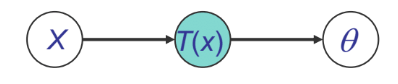
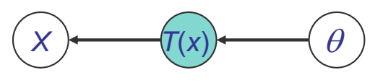
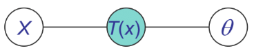
Sufficiency

We can see from above that for $p(x|\theta)$, $T(x)$ is sufficient for $\theta$ if there is no information in $X$ regarding $\theta$ beyond that in $T(x)$. Then, We can throw away $X$ for the purpose of inference w.r.t $\theta$. These could be shown by both Bayesian view and Frequentist view.

Bayesian view:

\[p(\theta|T(x),x)=p(\theta|T(x))\]

Frequentist view:

\[p(x|T(x),\theta)=p(x|T(x))\]

The Neyman factorization theorem:

$T(x)$ is sufficient for $\theta$ if

\[p(x,T(x),\theta) = \psi_1(T(x),\theta)\psi_2(x,T(x))\] \[p(x|\theta) = g(T(x),\theta)h(x,T(x))\]

Examples

Gaussian:

\[\eta = [\Sigma^{-1}\mu;-\frac{1}{2}vec(\Sigma^{-1})] = [\eta_1,vec(\eta_2)], \eta_1 = \Sigma^{-1}\mu, \eta_2 = -\frac{1}{2}\Sigma^{-1}\] \[T(x) = [x;vec(xx^T)]\] \[A(\eta)=\frac{1}{2}\mu^T\Sigma^{-1}\mu+\log{|\Sigma|}=-\frac{1}{2}tr(\eta_2\eta_1\eta_1^T)-\frac{1}{2}\log{(-2\eta_2)}\] \[h(x)=(2\pi)^{-k/2}\] \[\mu_{MLE}=\frac{1}{N}\sum_n T_1(x_n)=\frac{1}{N}\sum_n x_n\]

Multinomial:

\[\eta = [\ln(\pi_k/\pi_K);0]\] \[T(x) = [x]\] \[A(\eta) = -\ln(1-\sum_{k=1}^{K-1}\pi_k) = \ln(\sum_{k=1}^{K}e^{\eta_k})\] \[h(x) = 1\] \[\mu_{MLE}=\frac{1}{N}\sum_n x_n\]

Poisson:

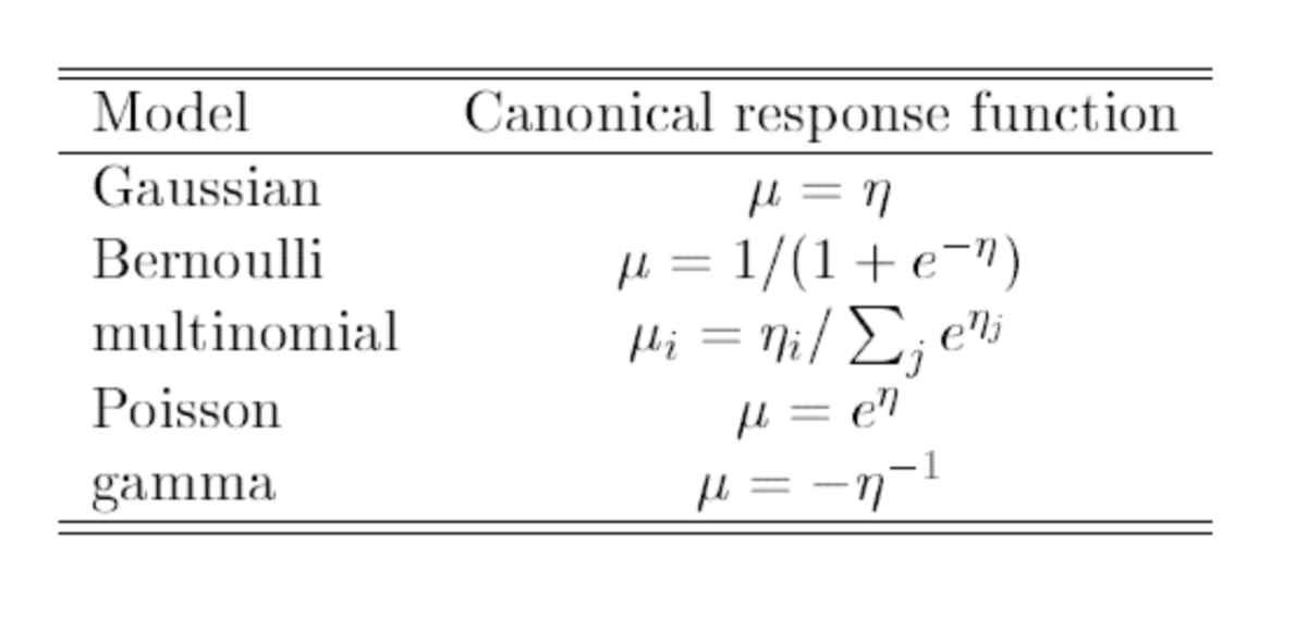
\[\eta = \log \lambda\] \[T(x) = x\] \[A(\eta) =\lambda = e^\eta\] \[h(x)=\frac{1}{x!}\] \[\mu_{MLE}=\frac{1}{N}\sum_n x_n\]

Generalized Linear Models

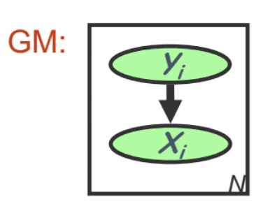
There are various conditional density estimation tasks that can be viewed as two-node GMs (see supplementary section for examples). Many are instances of Generalized Linear Models.

Generalized linear model (GLM) is a flexible generalization of ordinary linear regression that allows the linear model to be related to response variables via a link function, that have error distribution models other than a normal distribution. For example both linear regression and logistic regression can be unified by generalized linear model.

Commonality

We model the expecatation of $y$: $E_p(\mathbf{y)} = \mu = f(\theta^T\mathbf{x})$

$p$ is the conditional distribution of $y$
$f$ is the response function

The observed input $\mathbf{x}$ is assumed to enter into the model via a linear combination of its elements, and the conditional mean $\mu$ is represented as a function $f(\xi)$ of $\xi$, where f is known as the link function of $\xi=\theta^T\mathbf{x}$. The observed output $\mathbf{y}$ is assumed to be characterized by an exponential family distribution with conditional mean $\mu$.

Example 1: Linear Regression

Let’s take a quick recap on Linear Regression.

Assume that the target variable and the inputs are related by:

\[y_i = \theta^T x_i + \epsilon_i\]

where $\epsilon$ is an error term of unmodeled effects or random noise.

Now assume that $\epsilon$ follows a Gaussian distribution $N(0, \sigma)$, then

\[p(y_i|x_i;\theta) = \frac{1}{\sqrt{2\pi}\sigma}\exp(-\frac{(y_i -\theta^T\mathbf x_i)^2}{2\sigma^2})\]

We can use te LMS algorithm, which is a gradient ascent/descent approach, to estimate the parameter.

Example 2: Logistic Regression (sigmoid classifier, perceptron, etc.)

The condition distribution is a Bernoulli:

\[p(y|x) = \mu(x)^y (1-\mu(x))^{1-y}\]

where $\mu$ is a logistic function

\[\mu(x) = \frac{1}{1+e^{-\theta^T x}}\]

We can use the brute force gradient method as in LR. But we can also apply generic laws by observing the $p( y \vert x )$ is an exponential family function - a generalized linear model.

More examples: parameterizing graphical models

Markov random fields

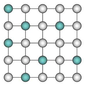
$p(\mathbf x) = \frac{1}{Z}\exp\{ -\sum_{c\in C} \phi_c(\mathbf x_c)\} = \frac{1}{Z}\exp\{-H(\mathbf x)\}$ $p(X) = \frac{1}{Z}\exp\{\sum_{i,j\in N_i}\theta_{ij}X_iX_j+\sum_i\theta_{i0}X_i\}$

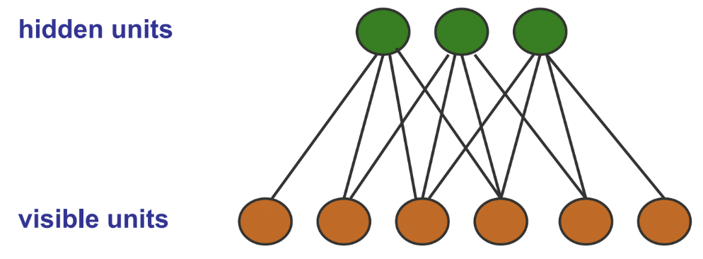
Restricted Boltzmann Machines

\[p(x,h|\theta) = \exp\{\sum_i \theta_i \phi_i(x_i)+\sum_j \theta_j \phi_j(x_j)+\sum_{i,j} \theta_{i,j} \phi_{i,j} (x_{i},h_j )-A(\theta)\}\]

Conditional Random Fields

Discriminative model, modeling $p(Y \vert X)$

$p_\theta(y \vert x) = \frac{1}{Z(\theta,x)}\exp\{\sum_c\theta_cf_c(x,y_c)\}$

$X_i$s are assumed as features that are inter-dependent
When labeling $X_i$, future observations are taken into account.

MLE for GLIMs

**Example canonical response functions**

Log-likelihood

\[\ell = \sum \limits_n \log h(y_n)+\sum \limits_n(\theta^Tx_ny_n-A(\eta_n))\]

Derivative is

\[\frac{d\ell}{d \theta}=\sum_n(x_ny_n-\frac{dA(\eta_n)}{\eta_n}\frac{d\eta}{d\theta})=\sum_nx_n(y_n-\mu_n)=X^T(y-\mu)\]

which is a fixed point function since $\mu$ is a function of $\theta$.

Iteratively Reweighted Least Squares (IRLS)

Recall that the Hessian matrix $H=-X^T WX$, and $\theta^*=(X^TX)^{-1} X^T y$ in least mean square optimization, we use Newton-Raphson method with cost function $\ell$:

\[\theta^{t+1}=\theta^t-H^{-1}\nabla_\theta\ell=(X^TW^tX)^{-1}X^TW^tz^t\]

where the response is:

\[z^t=X\theta^t+(W^t)^{-1}(y-\mu^t)\]

Hence, this can be understood as solving the Iteratively reweighted least squares problem. $\theta^{t+1}=arg\min_\theta(z-X\theta)^T(z-X\theta)$

Global and local parameter independence

Simple graphical models can be viewed as building blocks of complex graphical models. With the same concept, if we assume the parameters for each local conditional probabilistic distribution to be globally independent, and all nodes are fully observed, then the log-likelihood function can be decomposed into a sum of local terms, one per node:

\[\ell(\theta,D)=\log p(D|\theta)=\sum_i(\sum_n \log p(x_{n,i}|\mathbf{x_{n,\pi_i},\theta_i}))\]

Plate

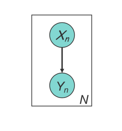
A plate is a macro that allows subgraphs to be replicated. Conventionally, instead of drawing each repeated variable individually, a plate is used to group these variables into a subgraph that repeat together, and a number is drawn on the plate to represent the number of repetitions of the subgraph in the plate.

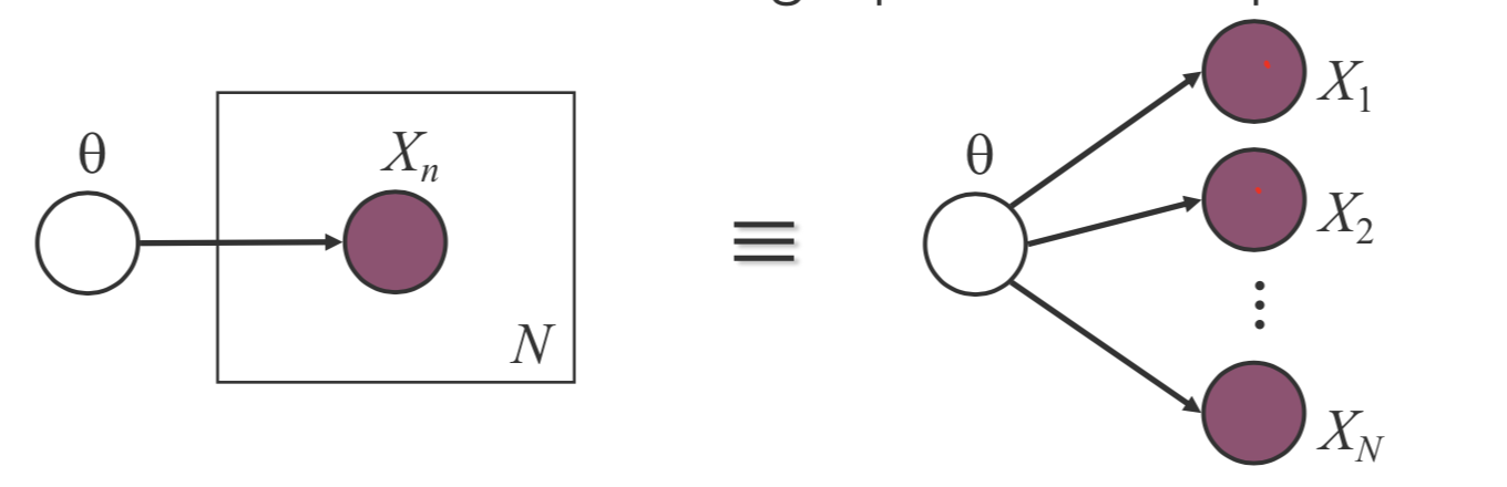
Rules for plates: Repeat every structure in a box a number of times given by the integer in the corner of the box (e.g. $N$), updating the plate index variable (e.g. $n$) as you go; Duplicate every arrow going into the plate and every arrow leaving the plate by connecting the arrows to each copy of the structure.

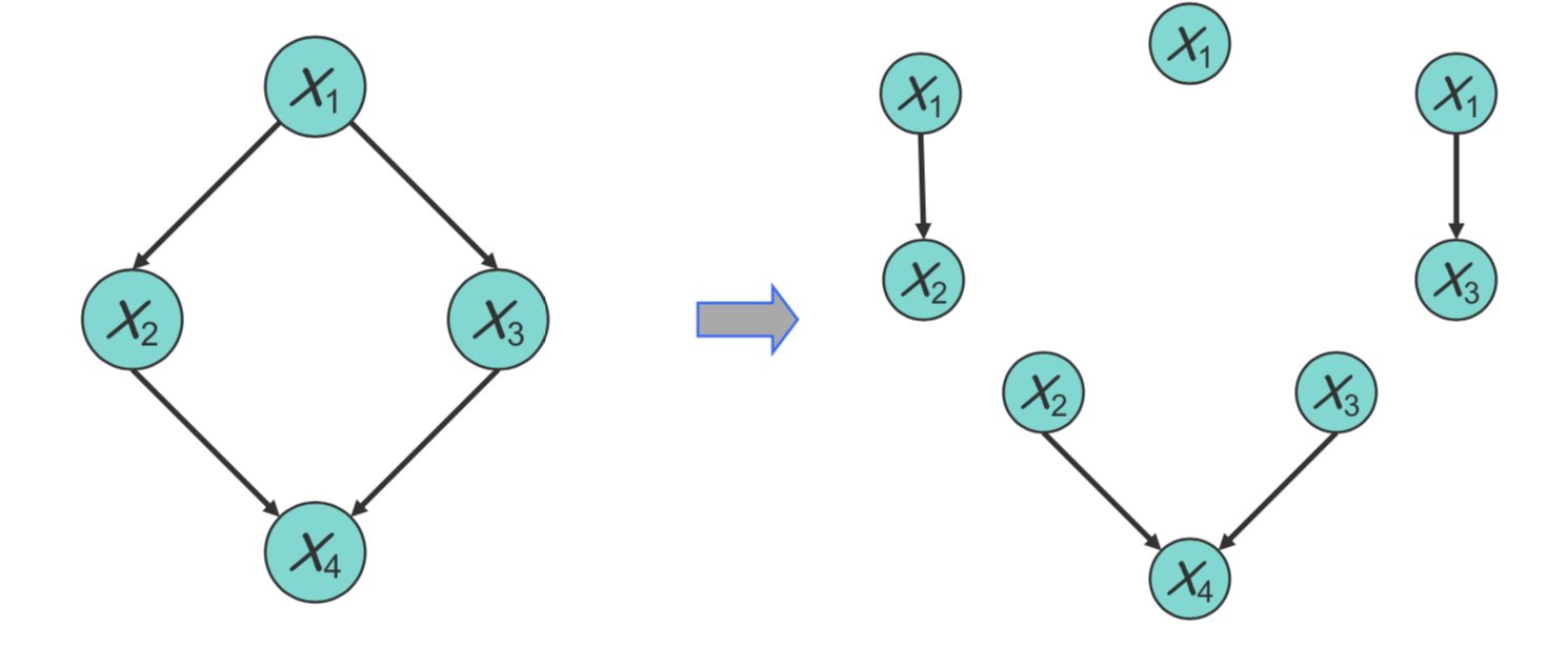
For example, in the directed acyclic network, it can be decomposed as $p(x|\theta)=\sum_{i=1}^np(x_i|\mathbf{x}_{\pi_i})=p(x_1|\theta_1)p(x_2|x_1,\theta_2)p(x_3|x_1,\theta_3)p(x_4|x_2,x_3,\theta_4)$ This is exactly like learning four separate small BNs, each of which consists of a node and its parents, as shown by the following graph:

Global parameter independence: For every DAG model, $p(\theta_m|G)=\prod_{i=1}\limits^Mp(\theta_i|G)$.

Local parameter independence: For every node, $p(\theta_i|G)=\prod_{i=1}^{q_i}p(\theta_{x_i^k|\mathbf{x}_{\pi_i}^j}|G)$.

Consider a network structure $G$ over a set of variables $X = \{X_1, \cdots, X_n\}$, parameterized by a set of parameters $\theta$. Each variable $X_i$ is associated with a CPD $P(X_i | U_i,\theta)$. Now, rather than assuming that each such CPD has its own parameterization $\theta_{X_i|U_i}$, we assume that we have a certain set of shared parameters that are used by multiple variables in the network. That is the global parameter sharing. Assuming $\theta$ is partitioned into disjoint subsets $\theta_1, \cdots, \theta_k$, and with each subset we assign a disjoint set of variables $\mathcal{V}_k\subset\mathcal{X}$. For $X_i\subset\mathcal{V_k}$, $P(X_i|\mathbf{U}_i,\theta)=P(X_i|\mathbf{U}_i,\theta^k)$ and for $X_i,X_j\subset\mathcal{V_k}$,

\[P(X_i|\mathbf{U}_i,\theta^k)=P(X_j|\mathbf{U}_j,\theta^k)\]

Supervised ML estimation

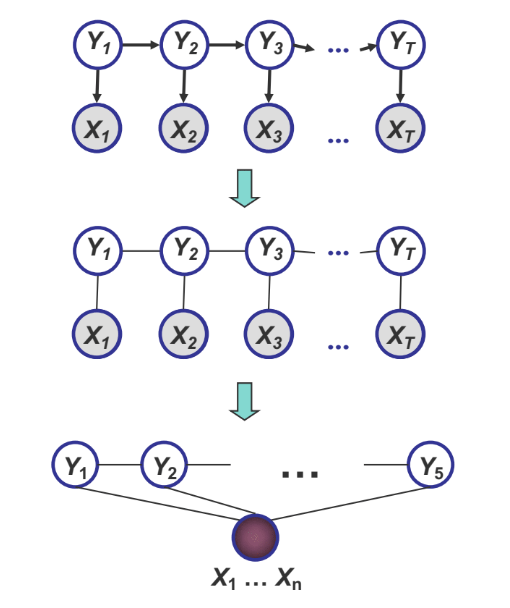
Hidden Markov Model (HMM)

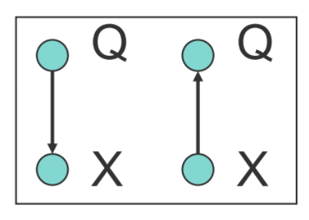
We are given a HMM, and let hidden states be $y_1, \cdots, y_N$, our observations be $x_1, \cdots, x_N$, which are all known to us.

In the training time, we can record the frequency of each transition from a hidden state to another, or from a hidden state to an observation state.

Let $A_{ij}$ be a transition from a hidden state $i$ to a hidden state $j$, and let $B_{ik}$ be a transition from a hidden state $i$ to an observation state $k$. We calculate our parameters using maximum likelihood estimation by the following:

\[a_{ij}^{ML} = \frac{\#transitions\ from\ i\ to\ j}{\#transitions\ from\ i\ to\ any\ hidden}\] \[b_{ik}^{ML} = \frac{\#transitions\ from\ i\ to\ k}{\#transitions\ from\ i\ to\ any\ observation}\]

If what we observe are continuous, we can treat them as Gaussian, and apply corresponding learning rules for Gaussian.

Pros

This method gives us the parameters that “best fit”, or maximizes the likelihood of seeing the training data. Therefore for the test data, intuitively it should be at least close to the truth. MLE tends to give good performance in the reality.

Cons

We just show that the parameters for calculation of probability upon seeing a test data depend on the frequency of seeing the same pattern in the training time. This leads to a problem. If there’s a test data case that’s never seen in the training data, then we will auto assign a zero probability to that test data, which is “infinitely wrong” because it will lead to a infinity cross entropy from real world to our model.

This also shows the overfitting problem, that we fit our training data too well that we cannot generalize our model to the real world well.

Example on the slide

$b_{F4}=0$ because there’s no casino roll such that $x=4$ and $y=F$ in the training data. However we all know this is not true!

Pseudocounts

To solve this problem, we can add “hallucinated counts” to all the cases, so that even the cases which are never seen in the training time will get some counts. Therefore at test time there will be no zero probability assigned to any case.

How many Pseudocounts do we add

Imagine if the total frequency of the cases in training is 100, and we add 10000 counts to one case, then that case will be assigned a very high probability in the test time. What we just have done is equal to saying that “I strongly believe this will happen”. In another word, we put lots of belief in that case.

However, if we just add one Pseudocount to each case, then the probability of frequent cases will decrease, but not too much. Their rankings in probability won’t change, because it’s just their denominators in MLE calculation have changed, by the same amount. The spared probability will be distributed to cases never seen in the training. They will be very small, but this eliminates the problem of zero probability in testing. This is what we call smoothing.

We can also see this as Bayesian Estimation under a uniform prior with “parameter strength”, while we add pseudocounts to cases.

Supplementary

Density Estimation

Density estimation can be viewed as single-node graphical models. It is the building block of general GM.

For density estimation we have:

MLE(maximum likelihood estimate)
Bayesian estimate

Discrete Distributions

Bernoulli distribution: $Ber(p)$

\[P(x)=p^x(1-p)^{1-x}\]

Multinomial distribution: $Multinomial(n,\theta)$

It’s generally similar to Binomial. However, the “1” in parameter indicates there will be only one trial. Therefore it’s similar to Bernoulli, except now we have $k$ instances that could happen, each with a probability $\theta_i$, where $\sum_{i=1}^{k}{\theta_i}=1$.

Suppose $n$ is the observed vector with:

\[n = \begin{bmatrix} n_1 \\ \cdots \\ n_k \end{bmatrix}, \sum_j n_j = N\] \[P(n)=\frac{N!}{n_1!n_2! \dots n_k!}\theta^n\]

MLE: constrained optimization with Lagrange multipliers

Objective Function:

\[l(\theta;D)=\sum_k{n_klog\theta_k}\]

constraint:

\[\sum_{k=1}^K{\theta_k=1}\]

Constrained cost function with a Lagrange multiplier:

\[l^-=\sum_k{n_klog\theta_k+\lambda(1-\sum_{k=1}^K{\theta_k})}\]

Bayesian estimation

Dirichlet prior:
$P(\theta)=C(\alpha)\prod_k{\theta_k^{\alpha_k-1}}$

Posterior distribution of $\theta$:
$P(\theta|x_1, \cdots, x_N)=\prod_k{\theta_k^{\alpha_k+n_k-1}}$

Posterior mean estimation:
$\theta_k=\frac{n_k+\alpha_k}{N+|\alpha|}$

Sequential Bayesian updating

Start with Dirichlet prior:
$P(\bar{\theta}|\bar{\alpha})=Dir(\bar{\theta}:\bar{\alpha})$

Observe N’ samples with sufficient statistics $\bar{n}'$. Posterior becomes:
$P(\bar{\theta}|\bar{\alpha},\bar{n}')=Dir(\bar{\theta}:\bar{\alpha}+\bar{n}')$

Hierarchical Bayesian Models

$\theta$ are the parameters for the likelihood $P(x \vert \theta)$

$\alpha$ are the parameters for the prior $P(\theta \vert \alpha)$

We can have hyper-parameters, etc.

We stop when the choice of hyper-parameters makes no difference to the marginal likelihood; typically make hyper-parameters constants.

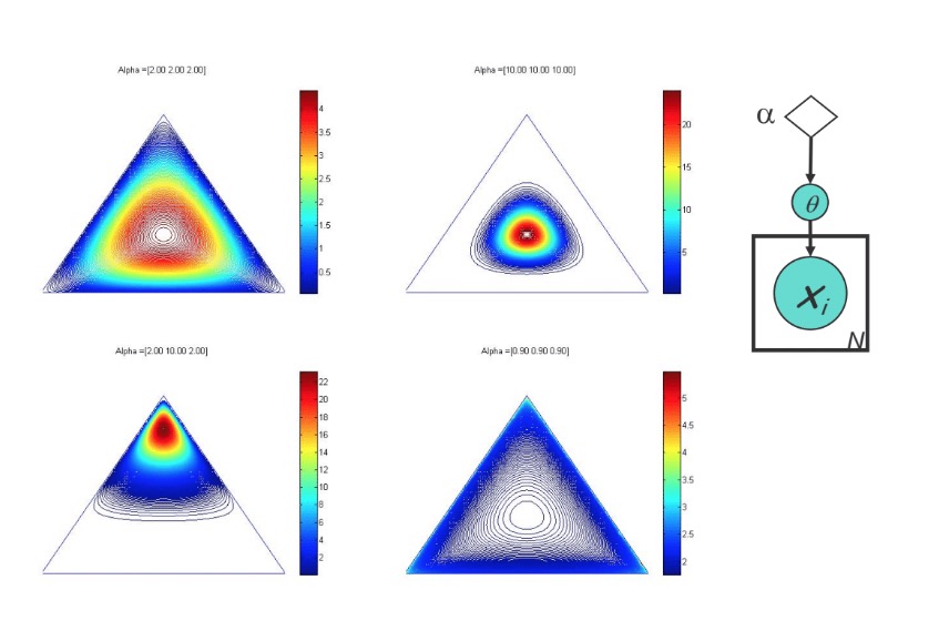
Limitation of Dirichlet Prior

Dirichlet prior could only put emphasis/bias on all coordinates or one single coordinate; it cannot, for example, emphasize two coordinates simultaneorly. The prior corresponding to different hyperparamter $\alpha$ is shown in the following picture:

The Logistic Normal Prior

Pro: co-variance structure
Con: non-conjugate

Continuous Distributions

Uniform Probability Density Function

$p(x) = \begin{cases} \frac{1}{b-a} & \ a \leq x \leq b \\ 0 & \ \text{elsewhere} \end{cases}$

Normal (Gaussian) Probability Density Function

$P(x)=\frac{1}{\sqrt{2\pi}\sigma}e^{-\frac{(x-\mu)^2}{2\sigma^2}}$

Multivariate Gaussian

$P(X;\bar{\mu},\sum)=\frac{1}{(\sqrt{2\pi})^\frac{n}{2}|\sum|^{\frac{1}{2}}}\exp(-\frac{1}{2}(X-\bar{\mu})^T\sum^{-1}(X-\bar{\mu}))$

MLE for a multivariate-Gaussian:

It can be shown that the MLE for $\mu$ and $\Sigma$ are:
$\mu_{MLE} = \frac{1}{N}\sum_n (x_n)$
$\Sigma_{MLE} = \sum_n (x_n - \mu_{MLE})(x_n - \mu_{MLE})^T = \frac{1}{N} S$

where the scatter matrix is:
$S = \sum_n (x_n - \mu_{MLE})(x_n - \mu_{MLE})^T = \sum_n x_n x_n^T - N \mu_{ML} \mu_{ML}^T$

Note that $X^TX=\sum_n{x_n x_n^T}$ may not be full rank (eg. if $N<D$), in which case $\sum_{ML}$ is not invertible

Bayesian Parameter Estimation for a Gaussian

Reasons for Bayesian Approach:

Update estimate sequentially over time
We may have prior knowledge about the expected magnitude of parameters
The MLE for $\Sigma$ may not be full rank if we don’t have enough data

Now that we only consider conjugate priors, and consider various cases of increasing complexity:

Known $\sigma$, unknown $\mu$
Known $\mu$, unknown $\sigma$
Unknown $\mu$ and $\sigma$

Unknown $\mu$, known $\sigma$

Normal Prior: $P(\mu | \mu_0, \tau^2) \sim \mathcal{N}(\mu_0, \tau^2) = \frac{1}{\sqrt{2\pi\tau^2t}}\exp\{ -\frac{1}{2\tau^2}(\mu-\mu_0)^2 \}$
Joint Probability: $P(x, \mu | \mu_0, \tau^2) = P(x | \mu) P(\mu) = (\frac{1}{\sqrt{2\pi\sigma^2}})^N \exp\{ -\frac{1}{2\sigma^2}\sum_{n=1}^N(x_n - \mu)^2 \} \frac{1}{\sqrt{2\pi\tau^2}}\exp\{ -\frac{1}{2\tau^2}(\mu-\mu_0)^2 \}$
Posterior:
$P(\mu | x, \mu_0, \tau^2) \sim \mathcal{N}(\tilde \mu, \tilde \sigma^2) = \frac{1}{\sqrt{2\pi \tilde \sigma^2}} \exp\{ - \frac{1}{2\tilde \sigma}(\mu-\tilde\mu)^2 \}$
where:
$\tilde \mu = \frac{N/\sigma^2}{N/\sigma^2 + 1/\tau^2} \bar{x} + \frac{1/\tau^2}{N/\sigma^2 + 1/\tau^2} \mu_0$
$\tilde \sigma^{-2} = \frac{N}{\sigma}^2 + \frac{1}{\tau^2}$
The posterior mean is a convex combination of sample mean and prior mean, and the posterior precision is the precision of the prior plus $1/\sigma^2$ of contribution for each observed data point.

Known $\mu$, unkown $\lambda = \sigma^{-2}$

Conjugate prior for $\sigma$: $P(\lambda | a, b)= \Gamma(a)^{-1}b^a\lambda^{a-1}\exp(-b\lambda)$
Joint Probability: $P(x, \lambda | a, b) = P(x | \lambda, a, b)P(\lambda | a,b ) = (2\pi)^{-n/2} \lambda^{n/2}\exp(-\frac{\lambda}{2}\sum_{n=1}^N(x_n - \mu)^2) \Gamma(a)^{-1}b^a\lambda^{a-1}\exp(-b\lambda)$
Therefore Posterior: $P(\lambda | x, a, b) \sim Gamma(\lambda | a_n, b_n) = \Gamma(a_n)^{-1}b_n^{a_n}\lambda^{a_n - 1} \exp(-b_n \lambda)$ where $a_n = a + \frac{n}{2}$ and $b_n = b +\frac{1}{2}\sum_{n=1}^N(x_n - \mu)^2$

Unkown $\mu$, unkown $\lambda$

Univariate Case
- Conjugate prior for $\mu$ and $\lambda = \sigma^{-2}$: (Normal-Inverse-Gamma)
  \[P(\mu, \sigma^2| m,V,a,b) = P(\mu | \sigma^2, m, V) P(\sigma^2 | a,b) = \mathcal{N}(\mu | m, \sigma^2 V) Gamma(\lambda | a_n, b_n)\]
Multivariate Case
- Conjugate prior for $\mu$ and $\Sigma$: (Normal-Inverse-Wishart)
  \[P(\mu, \Sigma |\mu_0, \kappa_0, \Lambda_0^{-1}, \nu_0) = P(\mu | \Sigma, \mu_0, \kappa_0) P( \Sigma | \Lambda_0^{-1}, \nu_0) = \mathcal{N}(\mu | \mu_0, \frac{1}{\kappa_0}\Sigma) \mathcal{IW}(\Sigma |\Lambda_0^{-1}, \nu_0)\]

Two nodes fully observed BNs

Conditional Mixtures
- Linear/Logistic Regression
Classification
- Generative and discriminative approaches

Classification

Goal: wish to learn $f: X \to Y$

Generative: Modeling the joint distribution of all data, i.e.: $P(x,y)$
Discriminative: Modeling only the conditional distribution, i.e.: $P(y \vert x)$

Conditional Gaussian

The data: $\{ (x_1,y_1),(x_2, y_2), \cdots, (x_n, y_n) \}$

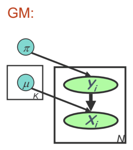
$y$ is a class indicator vector (one-hot encoding): $p(y_n) = multi(y_n; \pi) = \prod_{k=1}^K \pi_k^{y_{n,k}}$

$x$ is a conditional Gaussian variable with a class-specific mean: $p(x_n | y_{n,k} = 1, \mu, \sigma) = \frac{1}{\sqrt{2\pi\sigma^2}}\exp\{-\frac{1}{2\sigma^2}(x_n-\mu_k)^2 \}$

\[p(x|y, \mu, \sigma)=\prod_n p(x_n | y_n, \mu, \sigma) = \prod_n (\prod_k \mathcal{N} (x_n; \mu_k, \sigma_k)^{y_{n,k}} )\]

MLE of Conditional Gaussian

Data log-likelihood $l(\theta; D) = \log \prod_n p(x_n, y_n) = \log \prod_n p(y_n | \pi) p(x_n | y_n, \mu, \sigma)$
MLE:

$\hat \pi_{k, MLE} = \text{argmax}_{\pi} l(\theta; D) \Rightarrow \hat \pi_{k, MLE} = \frac{\sum_{n}y_{n,k}}{N} = \frac{n_k}{N}$, the fraction of sample of class $k$

$\hat \mu_{k, MLE} = \text{argmax}_{\mu} l(\theta; D) \Rightarrow \hat\mu_{k, MLE} = \frac{\sum_n y_{n,k} x_n}{\sum_n y_{n,k}} = \frac{\sum_{n} y_{n,k} x_n}{n_k}$, the average of samples of class $k$

Bayesian Estimation of Conditional Gaussian

Prior:
$P(\pi | \alpha) = Dirichlet(\pi; \alpha)$
$P(\mu_k | \nu) = \mathcal{N}(\mu_k; \nu, \tau^2)$
Posterior mean:

$\pi_{k, Bayes} = \frac{N}{N + \vert a \vert_1} \hat \pi_{k, MLE} + \frac{\vert a \vert_1}{N + \vert a \vert_1} \frac{a_k}{ \vert a \vert_1} = \frac{n_k + a_k}{N + \vert a \vert_1}$ where $\vert a \vert_1 = \sum_{k=1}^K a_k$

$\mu_{k, Bayes} = \frac{n_k/ \sigma^2}{n_k/\sigma^2 + 1/\tau^2}\hat{\mu}_{k, MLE} + \frac{1/\tau^2}{n_k/\sigma^2 + 1/\tau^2}\nu$, $\sigma_{Bayes}^{-2} = \frac{N}{\sigma^2} + \frac{1}{\tau^2}$

Gausian Distriminative Analysis:

Joint probability of a datum and its label is: $P(x_n, y_{n,k} = 1 | \mu, \sigma ) = p(y_{n,k} = 1) p(x_n | y_{n,k} = 1, \mu, \sigma) = \pi_k \frac{1}{\sqrt{2\pi \sigma^2}}\exp\{-\frac{1}{2\sigma^2}(x_n - \mu_k)^2 \}$
Predict the conditional probability of label given the datum: $p(y_{n,k} = 1 | x_n, \mu, \sigma) = \frac{\pi_k (2\pi\sigma^2)^{-1/2} \exp \{ -(x_n - \mu_k)^2 /2\sigma^2 \} }{\sum_{k'} \pi_{k'} (2\pi\sigma^2)^{-1/2} \exp \{ -(x_n - \mu_{k'})^2 /2\sigma^2 \} }$
Frequentist Approach: fit $\pi$, $\mu$ and $\sigma$ from data first
Bayesian Approach: compute the posterior dist. of the parameters first

Linear Regression

The data: $\{(x_1, y_1), (x_2, y_2), \cdots, (x_N, y_N) \}$, where $x$ is an input vector and $y$ is a response vector(either continuous or discrete)

A regression scheme can be used to model $p(y \vert x)$ directly rather than $p(x,y)$

A discrimintative probabilitstic model

Assume $y_i = \theta^T x_i + \epsilon_i$, where $\epsilon$ is an error term of unmodeled effects or random noise. Assume $\epsilon_i \sim \mathcal{N}(0, \sigma^2)$, then $p(y_i | x_i; \theta) \sim \mathcal{N}(\theta^Tx_i, \sigma^2) = \frac{1}{\sqrt{2\pi\sigma^2}} \exp\{ -\frac{1}{2\sigma^2} (y_i - \theta^Tx_i)^2 \}$

And by that each $(y_i, x_i)$ are i.i.d, we have: $L(\theta) = \prod_{i=1}^N p(y_i | x_i; \theta) = (\frac{1}{\sqrt{2\pi\sigma^2}})^N \exp\{ - \frac{1}{2\sigma^2}\sum_{i=1}^N(y_i - \theta^T x_i)^2 \}$

hence: $l(\theta) = n\log \frac{1}{\sqrt{2\pi\sigma^2}} - \frac{1}{2\sigma^2}\sum_{i=1}^N(y_i - \theta^Tx_i)^2$

we notice that maximizing this term w.r.t $\theta$ is equivalent to minimizing the MSE(mean square error): $J(\theta) = \frac{1}{2}\sum_{i=1}^N(x_i^T \theta - y_i)^2$

ML Structure Learning for Completely Observed GMs

Two “Optimal” Approaches

“Optimal” means the employed algorithms are guaranteed to return a structure that maximizes the objective. Some popluar heuristics, however, provide no gurantee on attaining optimality, interpretability or even do not have an explicit objective. e.g. structured EM, module network, greedy structural search, deep learning via auto-encoders, etc.

Will learn two classes of algorithms for guaranteed structure learning, albeit only applying to certain families of graphs:

Trees: The Chow-Liu Algorithm
Pairwise MRFs: covariance selection, neighborhood-selection

Structural Search

$O(2^{n^2})$ graphs over $n$ nodes
$O(n!)$ trees over $n$ nodes

But we can find exact solution of an optimal tree under MLE:

MLE score decomposable to edge-related elements
In a tree each node has only one parent

Lead to the Chow-Liu Algorithm

Chow-Liu Algorithm

\begin{aligned} l(\theta_G, G; D) &= \log P(D | \theta_G, G)\\ &= \log \prod_n (\prod_i p(x_{n,i} | x_{n, \pi_i(G)}, \theta_{i | \pi_i(G)} ) )\\ &= \sum_{i} (\sum_{n}\log p(x_{n,i} | x_{n, \pi_i(G), \theta_{i | \pi_i(G) }}) )\\ &= M\sum_i (\sum_{x_i, x_{\pi_i(G)}} \hat p(x_i, x_{\pi_i(G)}\log p(x_i | x_{\pi_i(G)}, \theta_{i | \pi_i(G)} ))\\ &= M\sum_i(\sum_{x_i, x_{\pi_i(G)}} \hat{p}(x_i, x_{\pi_i(G)}) \log \frac{\hat p(x_i, x_{\pi_i(G)}, \theta_{i | \pi_i(G)})}{\hat p(x_{\pi_i(G)}) \hat p(x_i) } ) - M \sum_i (\sum_{x_i} \hat p(x_i) \log \hat p(x_i))\\ &= M\sum_i \hat I(x_i, x_{\pi_i(G)}) - M \sum_i \hat H(x_i) \end{aligned}

For each pair of variable $x_i$ and $x_j$:
- Compute empirical distribution: $\hat p(x_i, x_j) = \frac{count(x_i, x_j)}{M}$
- Compute mutual information: $\hat I(x_i, x_j) = \sum_{x_i, x_j} \hat p (x_i, x_j) \log \frac{\hat p (x_i, x_j)}{\hat p (x_i) \hat p(x_j)}$
Define a graph with node $x_1, \cdots, x_n$:
- Edge $(i,j)$ get weight: $\hat I(x_i, x_j)$
- Compute maximum weight spanning tree
- Direction: pick any node as root, do BFS(breadth first search) do define directions, i.e.: we define an edge from node $A$ to node $B$ if we reach $B$ from $A$ in running BFS.

Structure Learning for General Graphs

Theorem: The problem of learning a BN structure with at most $d$ parents is NP-hard for any (fixed) $d \geq 2$.

Most structure learning approaches use heuristics

Exploit score decomposition:
- e.g: Greedy search through space of node-orders
- Local search of graph structures