Lecture 6: Learning Partially Observed GM and the EM Algorithm

Introduction to the process of estimating the parameters of graphical models from data using the EM (Baum-Welch) algorithm.

Introduction

In this previous lectures, we introduced the concept of learning Graphical Models from data, where learning is the process of estimating the parameters, and in some cases, the network structure from the data. Lecture 5 introduced this concept in the setting of completely observed GMs. Maximum likelihood estimation (MLE) in the setting of fully observed nodes and globally independent parameters for each conditional probability distribution is straightforward because the likelihood function can be fully decomposed as a product of independent terms, one for each conditional probability distribution in the network. This means that we can maximize each local likelihood function independently of the rest of the network, and then combine the solutions to get an MLE solution.

In this lecture, we turn our attention to partially observed graphical models, an equally important class of models including Hidden Markov Models and Gaussian Mixture Models. As we will see, in the presence of partially observed data, we lose important properties of the likelihood function: its unimodality, closed-form representation, and decomposition as a product of likelihoods for the different parameters. As a result the learning problem becomes substantially more complex, and we turn to the Expectation-Maximization algorithm to enable estimation of our model parameters.

Partially Observed GMs

Directed but partially observed GM

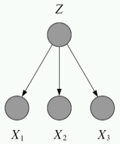
First consider the case of a fully observed, directed graphical model:

Fully observed, directed graphical model. In fully observed, i.i.d. settings,The log-likelihood function decomposes into a sum of local terms. We can maximize each local likelihood function independently.

\[\ell_c (\theta; D) = \text{log } p(x,z | \theta) = \text{log } p(z| \theta_z) + \text{log } p(x | z, \theta_x)\]

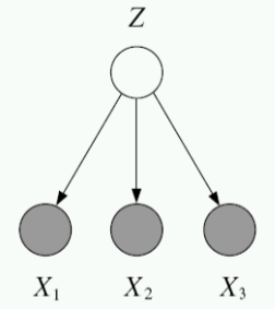
Compare this to the case of directed, but partially observed GMs. Suppose we now do not observe one of the variables, yet we would still like to write down the likelihood of the data. To do this, we marginalize (i.e. integrate or sum out) the unobserved probability.

Partially observed, directed graphical model. With unobserved or latent variables, the log-likelihood function no longer decomposes into a sum of local terms. All the parameters become coupled together via marginalization.

\[\ell_c (\theta; D) = \text{log } \sum_z p(x,z | \theta) = \text{log } \sum_z p(z| \theta_z) p(x | z, \theta_x)\]

Unobserved variables:

• A variable can be unobserved or latent because it is a(n):
  1. Abstract or imaginary quantity meant to simplifiy the data generation process, e.g. speech recognition models, mixture models.
  2. A real-world object that is difficult or impossible to measure, e.g. the temperature of a star, causes of disease, evolutionary ancestors.
  3. A real-world object that was not measured due to missed samples, e.g. faulty sensors.
• Discrete latent variables can used to partition or cluster data into sub-groups
• Continuous latent variables (factors) can be used for dimensionality reduction (e.g. factor analysis, etc)

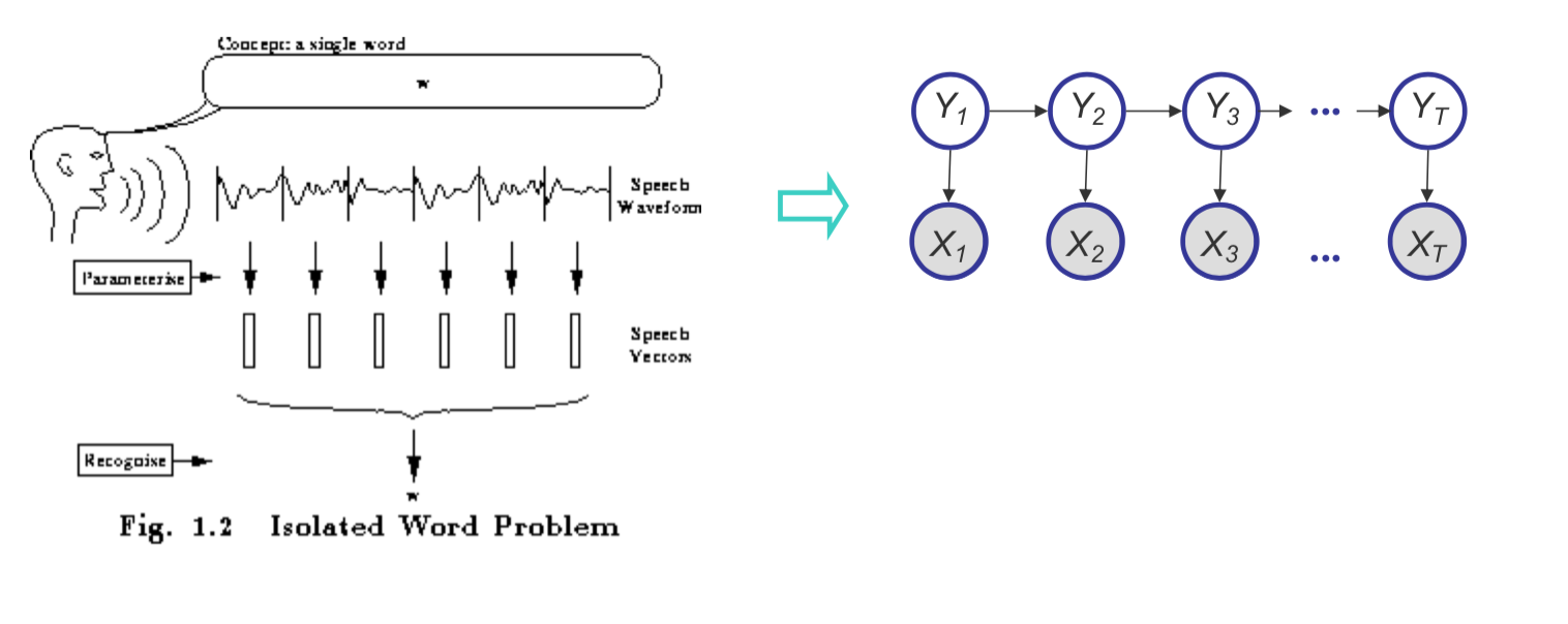
Example: HMMs for Speech Recognition

Our phones are capable of recognizing speech patterns and converting them to text. The initial approaches to this problem were based on Hidden Markov Models (HMMs). We assume there is a latent state that generates the noisy signal of speech that can be “chunked” into different components, or phonemes. We create dictionaries of different phonemes for different languages, and then we try to infer the sequence of phonemes that generated the speech.

An HMM used for speech recognition is a real-world example of a partially observed, directed graphical model. We try to infer the sequence of phonemes tat generated the noisy signal of speech.

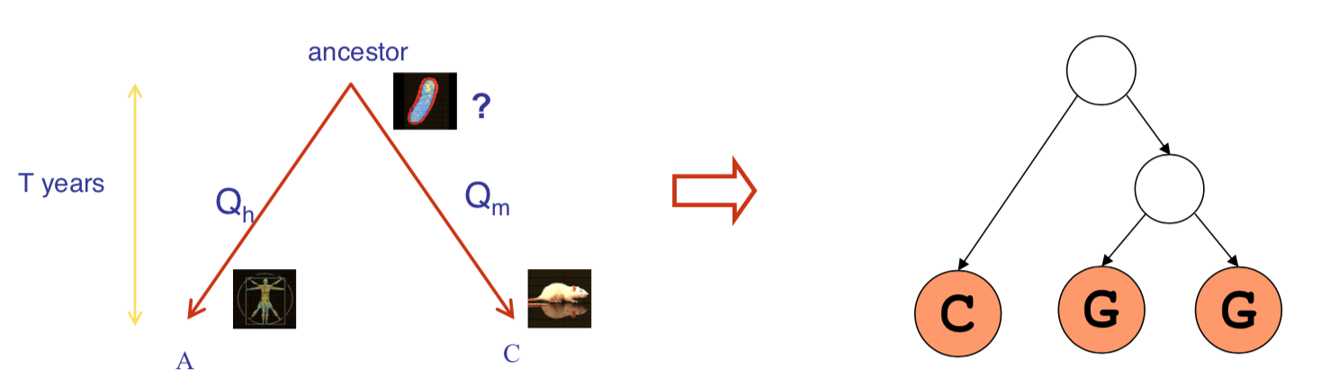
Example: A Baysian Network for Biological Evolution

This Baysian Network is not full observable . We cannot measure data from evolutionary ancestors no longer on earth, but they are still a useful latent variable for the model.

Probabilistic Inference

A GM $M$ describes a unique probability distribution $P$. To learn partially observable GMs, we must iterate between inferring relationships described by $P$ and estimating a plausible model $M$ from data $D$. In this way inference can be considered a subroutine of the learning problem:

Task 1. How do we answer queries about $P$, e.g. $P(X|Y)$?

• We use inference as a name for the process of computing answers to these queries.

Task 2. How do we estimate a plausible model $M$ from data $D$?

• We use learning as a name for the process of a obtaining point estimate of $M$. For the Bayesian approach, we seek $P(M|D)$ , which is also an inference problem.

There are many approaches for inference in GMs. They can be divided into two classes:

• Exact inference algorithms. Including the elimination algorithm, message-passing algorithm (sum-product, belief propagation), the junction tree algorithms. These algorithms can give the precise result of query. The major topic of this lecture is on exact inference algorithms.
• Approximate inference techniques. Including stochastic simulation / sampling methods, Markov chain Monte Carlo (MCMC) methods, variational algorithms. These algorithms only gives an approximate answer to the inference query. We will cover these methods in future lectures.

Mixture Models

A density model $p(x)$ may be multi-modal, but we may be able to model it as a mixture of uni-modal distributions (e.g. Gaussians). Suppose we have a dataset $x_n \in \mathbb{R}^D$ where $n=1$,…,$N$, and we believe the data has been generated from a mixture of $K$ Gaussian components. Let $z \in {1,…,K }$ be an unobserved random variable, such that $P(z = k) = \pi_k$, where $k = 1,…,K$. For $P(z)$ to be a valid probability distribution, $0 \leq \pi_k \leq 1$ and $\sum_{k=1}^K \pi_k =1$. We call $\pi_k$ the mixture proportion. Our assumption of the Gaussian components given a mixture label $k$ is expressed as $P(x| z=k) = N(x |\mu_k, \Sigma_k)$, where $\mu_k$ and $\Sigma_k$ are the parameters for each Gaussian component. Thus,

\[p(x_n) = \sum_z P(x | z) P(z) = \sum_{k=1}^K N(x | \mu_k, \Sigma_k) \pi_k\]

• $Z$ is a latent class indicator vector:

\[p(z_n) = \text{multi}(z_n | \pi) = \prod_k (\pi_k)^{z_n^k}\]

• $X$ is a conditional Gaussian variable with a class-specific mean/covariance:

\[p\parens{x_n | z_n^k = 1, \mu, \Sigma} = \frac{1}{\parens{2\pi}^{m/2} \abs{\Sigma_k}^{1/2}} \exp\parens{-\frac{1}{2} \parens{x_n - \mu_k}^T \Sigma_k^{-1} (x_n - \mu_k)}\]

A Gaussian Mixture Model is an example of a partially observed GM. A latent variable Z is introduced as a class indicator to separate a multi-modal distribution into simpler unimodal distributions.

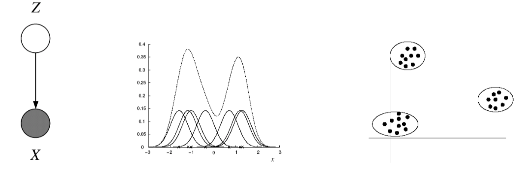
• The likelihood of a sample:

\begin{aligned} p(x_n | \mu, \Sigma) &= \sum_k p(z^k = 1 | \pi) p(x | z^k = 1, \mu, \Sigma) \\ &= \sum_{z_n} \prod_k ((\pi_k)^{z_n^k} N(x_n | \mu_k, \Sigma_k)^{z_n^k}) \\ &= \sum_k \pi_k N(x | \mu_k, \Sigma_k) \end{aligned}

MLE Solution for a Fully-Observed Gaussian Mixture Model

• The data log-likelihood can be decomposed when our latent variable $Z$ is also observed:

\begin{aligned} l (\theta | D) &= \text{log} \prod_n p(z_n , x_n) = \text{log} \prod_n p(z_n | \pi) p(x_n | z_n , \mu, \sigma_k)^{z_n^k} \\ &= \sum_n \text{log} \pi_k ^{z_n^k} + \sum_n \text{log} \prod_k N(x_n | \mu_k, \sigma_k)^{z_n^k} \\ &= \sum_n \sum_k z_n^k \text{log} \pi_k - \sum_n \sum_k z_n^k \frac{1}{2 \sigma_k^2} (x_n - \mu_k)^2 + C \end{aligned}

• Thus the MLE solution for the parameters can be found separately for these parameters:

\begin{aligned} \hat{\pi}_{k\text{, MLE}} &= \text{arg max}_{\pi} l(\theta | D) \\ \hat{\mu}_{k \text{, MLE}} &= \text{arg max}_{\mu} l(\theta | D) = \frac{\sum_n z_n^k x_n}{\sum_n z_n^k} \\ \hat{\sigma}_{k \text{, MLE}} &= \text{arg max}_{\sigma} l(\theta | D) \\ \end{aligned}

We do not typically have knowledge of $z_n^k$, the class labels. Clearly, it would be very easy to compute model parameters if that were the case! If we do not have knowledge of $z_n^k$, we cannot factorize the data log-likelihood or find the parameters independently (note also that the parameters here are all dependent on $z_n^k$).

Estimating the Parameters of a Partially-Observed GMM

What if we do not know $z_n$? We can use what is called the EM Algorithm or Expectation-Maximization algorithm to maximize the likelihood function for latent variable models. We can use this approach to find the maximum likelihood estimate of our model parameters when the original (hard) problem can be broken up into two (easy) pieces:

1. Estimate some “missing” or “unobserved” data from observed data and a current estimate of the parameters.
2. Using this “complete” data, find the maximum likelihood parameter estimates.

Thus we alternate between filling in the latent variables using the best guess (posterior) and updating the parameters based on this guess. So what does the EM algorithm look like for a GMM? Recall that estimate $\pi_k$, $\mu_k$, and $\Sigma_k$.

• The expected complete log likelihood:

\[\begin{aligned} \cross{ \ell_c (\theta \mid x,z)} &= \sum_n \cross{ \log p(z_n \mid \pi) }_{p(z|x)} + \sum_n \cross{ \log p(x_n | z_n, \mu, \Sigma) }_{p(z|x)} \\ &= \sum_n \sum_k \cross{ z_n^k } \log \pi_k - \frac{1}{2} \sum_n \sum_k \cross{ z_n^k } \parens{(x_n - \mu_k)^T \Sigma_k^{-1} (x_n - \mu_k) + \log \abs{ \Sigma_k } + C} \end{aligned}\]

We aim to maximize $ \langle \ell_c (\theta) \rangle $ iteratively using the following procedure.

1. Expectation Step: Computing the expected value of the sufficient statistics of the latent variables (e.g. $z$) given our current estimate of the parameters (i.e., $\pi$ and $\mu$).

\[\tau_n^{k(t)} = \langle z_n^k \rangle _{q^{(t)}} = p(z_n^k = 1 | x, \mu^{(t)}, \Sigma^{(t)}) = \frac{p(z_n^k = 1, x, \mu^{(t)}, \Sigma^{(t)})}{p(x,\mu^{(t)},\Sigma^{(t)})} = \frac{\pi_k^{(t)} N(x_n, | \mu^{(t)}, \Sigma^{(t)})}{\sum_i \pi_i^{(t)} N(x_n | \mu_i^{(t)}, \Sigma_i^{(t)})}\]

1. Maximization Step : Compute the parameters under current results of the expected value of the hidden variables:

\begin{aligned} \hat{\pi}_k &= \text{arg max} \langle \ell_c (\theta) \rangle &\implies \frac{\partial}{\partial \pi_k} \langle \ell_c(\theta) \rangle = 0, \forall k, \text{ s.t. } \sum_k \pi_k = 1\\ & &\implies \pi_k^{(t+1)} = \frac{1}{N} \sum_n \langle z_n^k \rangle _{q^{(t)}} = \frac{1}{N} \sum_n \tau_n^{k(t)} = \frac{1}{N} \langle n_k \rangle \\ \hat{\mu}_k &= \text{arg max} \langle \ell_c (\theta) \rangle &\implies \mu_k^{(t+1)} = \frac{\sum_n \tau_n^{k(t)} x_n}{\sum_n \tau_n^{k(t)}} \\ \hat{\Sigma}_k &= \text{arg max} \langle \ell_c (\theta) \rangle &\implies \Sigma_k^{(t+1)} = \frac{\sum_n \tau_n^{k(t)} (x_n - \mu_k^{(t+1)})(x_n - \mu_k^{(t+1)})^T}{\sum_n \tau_n^{k(t)}} \end{aligned}

This is isomorphic to MLE except that the variables that are hidden are replaced by their expectations. In the general formulation of the E-M algorithm they are replaced by their corresponding “sufficient statistics”.

Relationship to K-Means Clustering

Big picture: The EM algorithm for mixtures of Gaussians is like a “soft version” of the K-means algorithm. Suppose we have our dataset $x_n \in \mathbb{R}^D$ where $n=1$,…,$N$, and we would like to partition the data set into some $K$ clusters. Intuitively, we think of a cluster as a group of data points whose inter-point distances are small compared with the distances to points outside the cluster. $K$ is given, but we do not know the points are assigned each $k$ cluster. Let $\mu_k \in \mathbb{R}^D $ where $k=1,…,K$ be the centroid associated with the $k$th cluster. We define a hard cluster labeling $r_{nk}$, which is 1 if $x_n$ belongs to the $k$th cluster and otherwise $0$. Consider the objective function $J$:

\[J = \sum_{n=1}^N \sum_{k}^K r_{nk} || x_n - \mu_k ||^2\]

This non-convex objective function because we need minimize $J$ over both ${r_{nk}}$ and ${\mu_{k}}$. This can be solved by iterating:

• Minimize $J$ with respect to $r_{nk}$, keeping $\mu_k$ fixed. “E-step”
• Minimize $J$ with respect to $\mu_{k}$, keeping $r_{nk}$ fixed. “M-step”

Before iterating, we randomly initialize the centroid $\mu_k$ and covariance $\Sigma_k$ of each of the $K$ clusters. We then proceed to alternately perform the E- and M-steps until there is no further change in cluster assignments, or until some maximum number of iterations is exceeded.

1. “E-step” : We assign each data point to the closest cluster center using a hard assignment:

r_{nk} =\begin{cases} 1, & \text{if } k = \text{arg min}_j || x_n - \mu_j || ^2 \\ 0, & \text{otherwise.} \end{cases}

1. “M-step” : We set $\mu_k$ equal to the mean of all data points assigned to cluster $k$. Recall that the weights are either $0$ or $1$.

\[\frac{\partial J}{\partial \mu_k} = 2 \sum_{n=1}^{N} r_{nk} (x_n - \mu_k) = 0\] \[\implies \mu_k = \frac{\sum_{n=1}^N r_{nk} x_n }{\sum_{n=1}^N r_{nk}}\]

Each iteration reduces the objective funciton $J$, so the algorithm is guaranteed to converge, though not necessarily to a local optimum (recall that $J$ is non-convex).

Expectation-Maximization (E-M) Algorithm

Complete and Incomplete Log Likelihood

Complete Log Likelihood

Complete Log Likelihood is likelihood if both $x$ and $z$ are observed. Optimization given both $x$ and $z$ is straightforward MLE and can decompose into terms that can be independently maximized.

\[\ell_c (\theta; x,z) \vcentcolon= \log p(x,z \mid \theta) = \log p(x \mid \theta_x, z) + \log p(z \mid \theta_z)\]

Incomplete Log Likelihood

If $z$ is unobserved, we marginalize over $z$. We can no longer decouple into independent terms.

\[\ell_c(\theta;x) \vcentcolon= \log p(x \mid \theta) = \log \sum_{z} p(x,z \mid \theta)\]

Expected Complete Log Likelihood

Define the expected complete log likelihood for any distribution $z \sim q$. This function is a linear combination of $\ell_c$.

\[\langle \ell_c(\theta; x,z)\rangle_q \vcentcolon= \sum_z q(z \mid x, \theta) \log p(x,z \mid \theta) = \mathbb{E}_{q(z \mid x, \theta)} \log p(x,z \mid \theta)\]

The expected complete log likelihood can be used to create a lower bound on the incomplete log likelihood. The proof uses Jensen’s inequality ($\log \mathbb{E}[x] \ge \mathbb{E}[ \log x]$). The proof also uses the importance sampling trick ($\mathbb{E}_p[ f(x)] = \mathbb{E}_q[ \frac{f(x)p(x)}{q(x)}] $).

\[\begin{aligned} \ell(\theta, x) &= \log p(x \mid \theta) \\ &= \log \sum_z p(x,z \mid \theta) \\ &= \log \sum_z \frac{q(z \mid x)}{q(z \mid x)} p(x,z \mid \theta) & \text{importance sampling trick}\\ &= \log \sum_z q(z \mid x) \frac{p(x,z \mid \theta) }{q(z \mid x)} & \log \mathbb{E}_q[\ldots]\\ &\ge \sum_z q(z \mid x) \log \frac{p(x,z \mid \theta)}{q(z \mid x)} & \text{Jensen's } \mathbb{E}_q [\log \ldots] \\ &= \mathbb{E}_q [\log p(x,z \mid \theta)] - \mathbb{E}_q \log q(z \mid x)\\ \ell(\theta, x) &\ge \langle \ell_c(\theta; x,z) \rangle_q + H_q \end{aligned}\]

The second term $H_q$ is the entropy of $q(z \mid x)$. A distribution is $[0,1]$, so the log of a distribution is $\langle -\infty,0 \rangle$, which is why the constant $H_q$ is positive. Because $H_q$ is positive and does not depend on $\theta$, we can try to maximize $\langle \ell_c(\theta; x,z)\rangle_q$ to maximize a lower bound on $\ell(\theta, x)$.

Lower Bounds and Free Energy

For fixed data $x$ define a functional called the free energy. This is the term $\langle\ell_c(\theta; x,z)\rangle_q + H_q$ from the above proof.

\[F(q,\theta) \vcentcolon= \sum_z q(z \mid x) \log \frac{p(x,z \mid \theta)}{q(z \mid x)} \le \ell(\theta; x)\]

We can perform EM algorithm (generally MM algorithm) on $F$:

• E-step: $q^{t+1}=\text{arg max}_q F(q, \theta^t)$
• M-step: $\theta^{t+1}=\text{arg max}_\theta F(q^t, \theta)$

E-step

The E-step is a maximization over the posterior over latent variables given data and parameters $q(z \mid x, \theta)$.

\[q^{t+1}=\text{arg max}_q F(q, \theta^t)\]

If $q$ is the optimal posterior $p(z \mid \theta^t, x)$, this maximization attains the bound $\ell(\theta^t; x)$. The proof uses an application of the Bayes rule $p(x,z \mid \theta^t)=p(x \mid \theta^t) p(z \mid x, \theta^t)$.

\[\begin{aligned} F(p(z\mid x,\theta^t), \theta^t) &= \sum_z p(z \mid x, \theta^t) \log \frac{p(x,z \mid \theta^t)}{p(z \mid x, \theta^t)}\\ &= \sum_z p(z \mid x, \theta^t) \log \frac{p(x \mid \theta^t) p(z \mid x, \theta^t)}{p(z \mid x, \theta^t)} & \text{Bayes rule}\\ &= \sum_z p(z \mid x, \theta^t) \log p(x \mid \theta^t) \\ &= \log p(x \mid \theta^t) \sum_z p(z \mid x, \theta^t) & \text{term does not depend on $z$}\\ &= \log p(x \mid \theta^t) & \text{sum of distribution is 1}\\ &= \ell(\theta^t; x) \end{aligned}\]

M-step

The M-step is a maximization over the parameters given data and latent variables. As discussed previously, the free energy breaks into two terms, one of which ($H_q$) does not depend on $\theta$. Therefore we only need to consider the first term during the M-step.

\[F(q,\theta) = \langle \ell_c(\theta;x,z)\rangle_q + H_q\] \[\theta^{t+1}=\operatorname{argmax}_\theta F(q^t, \theta) =\operatorname{argmax}_{\theta} \langle \ell_c(\theta;x,z)\rangle_{q^t}\]

If $q^t = p(z \mid x, \theta)$, this is equivalent to fully observable MLE where statistics are replaced by their expectations w.r.t. $ p(z \mid x, \theta)$. We are minimizing the expected loss over the distribution $p$.

Example: Hidden Markov Models & Baum-Welch Algorithm

An example Hidden Markov Model which has been unrolled to T timesteps.

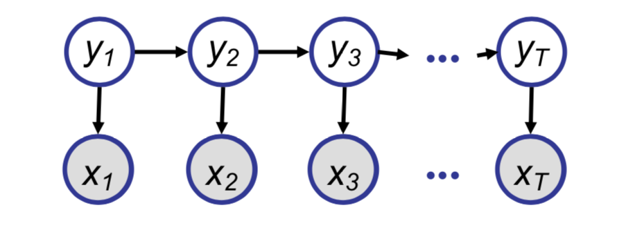
Hidden Markov Models (HMMs) are one of the common ways of modeling time series data. It is used in traditional speech recognition systems, natural language processing, computational biology etc. HMMs allow us to deal with both observed and hidden events. Most of the common HMMs follow the first order markov assumption, which states that, when predicting the future the past doesn’t matter, only the present. If there is a sequence of states $q_1,q_2,…q_i$, then the first order markov assumption says that

\[P(q_i=a|q_1,q_2,..q_{i-1}) = P(q_i=a|q_{i-1})\]

Hidden Markov Model Definitions

An HMM is specified in following components

• A set of N states, $\mathbf{y} = y_1,y_2,…,y_N$
• Transition probability between any two states

\[\begin{aligned} p(y_t^j=1|y_{t-1}^i = 1) &= a_{i,j} = \mathbf{A}, \text{or} \\ p(y_t^j=1|y_{t-1}^i = 1) &\sim \texttt{Multinomial}(a_{i,1},\ldots,a_{i,m}), \forall i \in I \end{aligned}\]

• Output observations, $\mathbf{x} = x_1, x_2,\ldots,x_T $

• Emmision Probabilities, the probability of an observation being generated from a state.

\[p(x_t|y_t^i=1) \sim \texttt{Multinomial}(b_{i,1},\ldots,b_{i,K}), \forall i \in I\]

• Start or prior probabilities

\[p(y_1) \sim \texttt{Multinomial}(\pi_1,\ldots,\pi_m)\]

EM for Hidden Markov Models

For an HMM with $N$ hidden states and with $T$ observations, computing the total observation likelihood would be computationally expensive, as there are $N^T$ sequences. This can be computed efficiently using the Baum-Welch algorithm, also known as the forward-backward algorithm.

• The complete log likelihood

\[\begin{aligned} l_c(\mathbf{x},\mathbf{y};\theta) &= \log p(\mathbf{x},\mathbf{y};\theta) \\ &= \log \prod_n (p(y_1^n) \prod_{t=2}^T p(y_t^n | y_{t-1}^n) \prod_{t=1}^T p(x_t^n | y_t^n)) \end{aligned}\]

• The expected complete log likelihood

\[\begin{aligned} \cross{ l_c(\theta; \mathbf{x},\mathbf{y}) } &= \log p(\theta;\mathbf{x},\mathbf{y}) \\ &= \sum_n \parens{\cross{y_{n,1}^i}_{p(y_{n,1} \mid x_n} \log \pi_i } + \sum_n \sum_{t=2}^T \parens{ \cross{y_{n,t-1}^i, y_{n,t}^j}_{p(y_{n,t-1}, y_{n,t} \mid x_n} \log a_{i,j}} + \sum_n \sum_{t=1}^T \parens{x_{n,t}^k \cross{y_{n,t}^i}_{p(y_{n,t}\mid x_n} \log b_{i,k}} \end{aligned}\]

• Expectation Step : Fix $\theta$ and compute the marginal posterior

\[\begin{aligned} \gamma_t^n &= \langle y_t^n \rangle = p(y_t = i | \mathbf{x}; \theta), \\ \xi_t^n &= \langle y_t^n y_{t-1}^n \rangle = p(y_t = i , y_{t-1} = j | \mathbf{x}; \theta) \\ \end{aligned}\]

• Maximization Step : Update $\theta$ by MLE

\[\begin{aligned} \pi^{ML} &= \frac{\sum_n \gamma_1^n}{N} \\ \mathbf{A}^{ML} &= \frac{\sum_n \sum_{t=2}^T \xi_t^n}{\sum_n \sum_{t=1}^{T-1} \gamma_t^n} \\ b^{ML} &= \frac{\sum_n \sum_{t=2}^T \xi_t^n}{\sum_n \sum_{t=1}^{T-1} \gamma_t^n} \end{aligned}\]

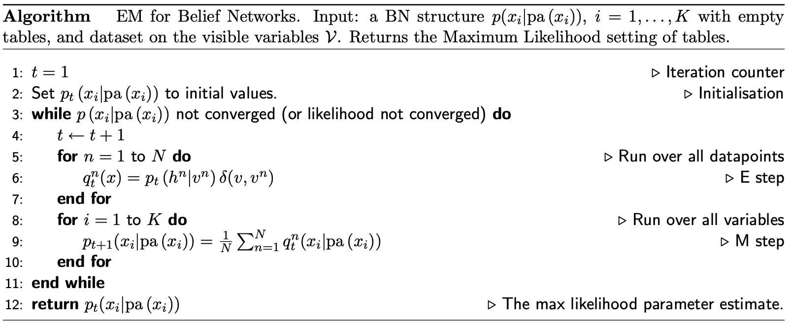
Example: EM for a general BN

For a general bayesian network $p(x) = \Pi_i p(x_i | \texttt{pa}(x_i))$ where $\texttt{pa}(x_i)$ are the parents of the node $x_i$, the expectation maximization algorithm can be written as

See section 11.2.4 of David Barber’s book for more details of this algorithm

Example: EM for conditional mixture models

For example we will model $p(Y \mid X)$ using different experts for different regions of $X$. Our selection of experts is the latent variable $z$. The model of $p(y \mid x)$ is that an expert is selected based on $x$ and that expert produces a regression based on $x$.

\[p(y \mid x) = \sum_k p(z^k=1 \mid x, \chi)p(y \mid z^k=1,x,\theta_i,\sigma)\]

• Latent variable $Z$ selects expert using softmax for normalization (softmax guarantees output is a distribution)

\[P(z^k=1 \mid x)=\operatorname{softmax}(\chi^Tx)\]

• Each expert is a linear regression. The output distribution has variance $\sigma_k^2$ and mean $\theta_k^Tx$.

\[P(y \mid x, z^k=1) = \eta(y;\theta_k^Tx, \sigma_k^2)\]

• Posterior expert responsibilities assigning points to experts are

\[p(z^k=1 \mid x,y,\theta) = \frac{p(z^k=1 \mid x) p_k(y \mid x, \theta_k, \sigma_k^2)}{\sum_j p(z^j=1 \mid x) p_j(y \mid x, \theta_j, \sigma_j^2)}\]

• Using the expected complete log likelihood as loss

\[\begin{aligned} \langle \ell_c(\theta; x,y,z) \rangle &= \sum_n \langle \log p(z_n \mid x_n, \chi) \rangle_{p(z \mid x, y)} + \sum_n \langle \log p(y_n \mid x_n, z_n, \theta, \sigma) \rangle_{p(z \mid x,y)} \\ &= \sum_n \sum_k \langle z_n^k \rangle \log \big( \operatorname{softmax}(\chi_k^Tx_n)\big) - \frac{1}{2} \sum_n \sum_k \langle z_n^k \rangle \Big( \frac{y_n-\theta_k^Tx_n}{\sigma_k^2} + \log \sigma_k^2 + C \Big) \end{aligned}\]

The resulting EM algorithm:

• E-step calculates the responsibilities \(\tau_n^{k(t)}=p(z_n^k=1 \mid x_n,y_n, \theta) = \frac{p(z_n^k=1 \mid x_n)p_k(y_n \mid x_n, \theta_k, \sigma_k^2)}{\sum_j p(z_n^j=1 \mid x_n)p_j(y_n \mid x_n, \theta_j, \sigma_j^2)}\)
• M-step calculates linear regressions for each expert, each data point weighted by the expert’s responsibility (see homework)

EM Variants

• Partially Hidden Variables: We can use EM when there are missing (hidden) variables in some cases and not in others. In the E-Step we can estimate the hidden variables for only the incomplete cases. The M-step then optimizes the log-likelihood on the complete data plus the expected likelihood of the incomplete data found using the E-step.
• Sparse EM: In this variant, you do not exactly re-compute the posterior probability on each data point under all models, because it is practically zero. Instead, you keep an “active list” which you update every once in a while.
• Generalized (Incomplete) EM: It might be hard to find the ML parameters in the M-step, even given the completed data. We can still make progress by doing an M-step that improves the likelihood a bit (e.g. gradient step). Recall the IRLS step in the mixture of experts model.

Summary

Learning the parameters of partially observed graphical models, or latent variable models, is considerably more difficult than for fully observed GMs. This is because the unobserved or latent variables tie the observed variables together via marginalization, and we can no longer decompose the maximum likelihood function into independent conditional probabilities.

The EM Algorithm provides a way of maximizing the likelihood function for latent variable models. We can find the MLE parameters when the original problem can be broken into 2 steps: (1) Estimating or “filling in” the unobserved latent variables using the best guess (posterior) provided from our observed data and current parameters, and (2) updating the parameters based on this guess:

E-Step

\[q^{(t+1)} = \text{arg max}_q F(q, \theta^t)\]

M-Step

\[\theta^{(t+1)} = \text{arg max} _{ \theta} F(q^{(t+1)}, \theta ^t)\]

• EM Pros:
  • No learning rate (step-size) parameter. It is possible that one or both minimizations can be computed analytically.
  • Automatically enforces parameter constraints. Problems can be subdivided into discrete and continuous optimization problems.
  • Very fast for low dimensions. Each minimization can be computed quickly and analytically.
  • Each iteration guaranteed to improve the likelihood
• EM Cons
  • Can get stuck in local minima. Even if both subproblems are convex does not mean that iteratively solving both reaches a global minimum.
  • Can be slower than conjugate gradient (especially near convergence). Each subproblem is solved from scratch in each iteration as opposed to an iterative method that refines a solution. We solve for $\theta$ given current $q$ ignoring current $\theta$, then solve for best $q$ given $\theta$ ignoring the current $q$.
  • Requires computationally expensive inference step
  • Is a maximum likelihood/MAP method

Additional Resources

• Jordan textbook, Ch. 11
• Koller textbook, Ch. 19.1-19.4
• Borman, The EM algorithm (A short tutorial)
• Variations on EM algorithm by Neal and Hinton