Lecture 7: Maximum likelihood learning of undirected GM
Algorithms for learning UGMs along with a brief overview of CRFs.
Introduction and IPF
MLE for undirected graphical models
We have an undirected graphical model and we know that using the Hammersley–Clifford theorem that it can be represented by a Gibbs distribution. Now the question arises if we can follow the sane procedure as for directed graphical Models to find the MLE of an UGM? The answer is no - we cannot. This is because for directed graphical models the log likelihood decomposes into a sum of terms, one per family i.e. (node + it’s parents). However the same is not applicable to undirected graphical models, as there is a normalization constant $Z$ that is a function oaf all the parameters and thus the probability distribution does not split into a sum of terms.
Although this is a big drawback, we still use undirected graphical models as they are useful - they are used to represent some special cases which cannot be represented by directed graphical models alone. The next section outlines the procedure for finding the MLE through taking the derivative of the log-likelihood and the difficulties that arise by doing so.
Log Likelihood for UGMs
Here, we introduce two new quantities Total Count and Clique Count. Total Count for an Undirected Graphical Model $(V, E)$, is simply the number of times that a configuration x (i.e., $X_v = x$) is observed in a dataset $D = \left{ \mathbf { x } _ { 1 } , \ldots , \mathbf { x } _ { N } \right}$
The Clique Count is expressed as a marginal of the Total Count.
Using the counts to express the log likelihood we have,
Taking the derivative we get, The first is fairly simple
The second term however is a little more involved,
Putting the first and second terms together, the derivative becomes
Equating to zero and solving we get,
Notice that the $\psi _ { c } \left( \mathbf { x } _ { c } \right)$ term gets cancelled and we are left with a condition. In other words, at the maximum likelihood setting of the parameters, for each clique, the model marginals must be equal to the observed marginals (empirical counts). This doesn’t tell us how to get the ML parameters, it just gives us a condition that must be satisfied when we have them.
Thus we turn to two important algorithms, which we call the workhorse algorithms.
Iterative Proportional Fitting
We have from the derivative of the likelihood this relationship that,
Now since $\psi _ { c } \left( \mathbf { x } _ { c } \right)$ turns up on both sides of the equation, solving it in the closed form is impossible. We can however treat this as a fixed point iteration by treating the one on the left hand side as being ahead (uknown) and the one on the right as known, we can then estimate the one on the left with the one on the right using the equation. We cycle through all the cliques and iterate,
IPF, is also a co-ordinate ascent algorithm, where the co-ordinates are the parameters of the clique potentials. During each step of the algorithm the log-likelihood increases and thus it will converge to a global maximum.
Information-theoretic viewpoint on IPF
Maximizing the log likelihood is equivalent to minimizing the KL divergence from the observed distribution to the model distribution.
Generalized Iterative Scaling (GIS): Introduction
Now this second algorithm is where we start thinking more about feature-based models. So far, when we mention potential functions, we feel that it is trivial. Either you learn it, or you simply specify numbers at will. But there are some problems. To illustrate this, let’s take a look at a real task of spell checking. One of the most useful and powerful devices in spell checking is to build affinity models of character strings.
Feature-based Clique Potentials
For example, if we were to look at the consecutive appearance of 3 characters, $c_1, c_2, c_3$, which we represent with the potential function $\psi(x_c)$. The rationale behind this is that we can use this to score the likelihood of misspelling. E.g. If we see the sequence ‘zyz’, we would know that such a sequence does not exist in the English vocabulary and therefore has a very high likelihood of being a misspelling. On the other hand, if we see the sequence ‘ink’, we know that there are some words which contain this sequence and consequently a lower likelihood of misspelling. This is an example of how the potential can help us do spell checking. However, if we were to iterate over all the different combinations of triplets in the alphabet, this would imply that we have $26^3$ features, and this gets worse if we increase the size of the sequence. Such a general “tabular” potential function would be exponentially costly for inference and have exponential numbers of parameters that we must learn from limited data, which would exhaust the computer’s memory.
One solution is to change the graphical model to make cliques smaller. But this changes the dependencies, and may force us to make more independence assumptions than we would like. Another solution is to keep the same graphical model, but use a less general parameterization of the clique potentials. And this is the idea behind feature-based models.
Features: In our earlier example of spell checking, since we know how frequent certain triplets are based on the existing knowledge (e.g. a dictionary or our own vocabulary), we can pick out those we have the greatest confidence in and assign them features. Here a feature is defined as a function which is vacuous for most joint settings except a few particular ones, in which it returns either high or low values. E.g. we can define a feature $f_{ing} = 10$ and $f_{ate} = 9$, and so on and so forth. By the time we get to the 50th or 100th feature, we assume that these combinations are less likely and assign them some arbitrary small likelihood of $\alpha$. We can also define features when the inputs are continuous. Then the idea of having a cell on which the feature is active is no longer relevant, but we might still have a compact parameterization of the feature.
This is a different approach from deep learning where we become overcomplete and hope that the big data will funnel in to get these numbers into place, with no guarantee, because we don’t know how much data is necessary to get the numbers into place, i.e. we don’t know the sample complexity. Instead, here we have a way in which we utilize human knowledge to build a model. And even today, the most successful speech recognition models have their foundations based on this concept.
Features as Micropotentials: Let’s move on to the details. By exponentiating them, each feature function can be made into a “micropotential.” We can multiply these micropotentials together to get a clique potential. For example, a clique potential $\psi(c_1,c_2,c_2)$ could be expressed as:
There’s still a potential over $26^3$ possible settings, but only uses $K$ parameters if there are $K$ features, and by having one indicator function per combination of $x_c$, we recover the standard tabular potential.
Combining Features: Note that these features can be handcrafted. We also append weights $\theta_k$ in the function because we do not have contextual knowledge of how important each feature is. The marginal over the clique is a generalized exponential family distribution, actually, a GLIM:
In general, the features may be overlapping, unconstrained indicators or any function of any subset of the clique variables. For example if you have multiple cliques such as overlapping windows over all possible combinations of triplets in our spelling checking example, this does not changed the anatomy of the potential, where we still have a weighted sum of the features.
Feature Based Model: We can multiply these clique potentials as usual:
However, in general, we can forget about associating features with cliques and just use a simplified form:
With this redesign, we have the exponential family model, with the features as sufficient statistics. And so we get compactness and prior knowledge. However, the difficulty of learning is greater. Recall that in IPF, we have:
All we know is that the entire thing can be reweighted, iteratively, but here we have a combination of $\theta$ and $f$, and it is not obvious how we may use this rule to update the weights and features individually.
MLE of Feature Based UGMs: Here let us look at our loss function (scaled likelihood):
We introduce $N$ to allow the introduction of an empirical distribution. This is a technicality we can put aside, because $N$ is a constant and does not change the relative numbers in our estimate. The loss function breaks down into two terms where one is a naive sum of $\theta f(x)$, and the other is the more complex $\log Z(\theta)$ with $\theta$ buried deeply into a compound. This is something that we cannot easily take the derivative with respect to.
So instead of attacking this objective directly, we attack its lower bound. The rationale is that often in machine learning we linearize what is non-linear to reduce the complexity. Here we make use of the property that
This bound holds for all $\mu$, in particular, it also holds for $\mu = Z^{-1}(\theta^{(t)})$. As a result, we have
Where we assume that there exists a previous version $\theta^{(t)}$.
Generalized Iterative Scaling: Algorithm
To make our task more explicit, let us establish an explicit relationship; the desired version of $\theta$ versus the current version of $\theta$, called $\Delta\theta$, such that $\Delta \theta_i^{(t)} := \theta_i - \theta_i^{(t)}$. We substitute this into the lower bound of the scaled log-likelihood.
Unfortunately, this is still a difficult expression to deal with. Here $\theta$ is compounded by the summation over all $\theta$, and then exponentiated. It becomes non-linear, and every $\theta$ is coupled with every other $\theta$ because of this operation. But this function has a specific form. It is the exponential of a sum or weighted sum. Let’s switch perspective and treat $f$ as the weights and $\Delta \theta$ as the arguments.
With the assumptions
The convexity of the exponential is such that
And now we have the sum of the exponentials of each individual $\theta$. This is a commonly used algebraic trick in machine learning.
This is known as GIS. So instead of using the original scaled log-likelihood, we use the lower bound of that which we call $\Lambda (\theta)$. Subsequently we can then take the following standard steps.
Take derivative:
Set the derivative to zero
Where $p^{(t)}(x)$ is the unnormalized version of $p(x \mid \theta^{(t)})$
We now have the update equations
Why do we call this scaling? To see this, take a look at the form of the last equation. It is in the form of a ratio calculated over two methods. One is the feature weighted by its empirical probability, and the other is a feature weighted by the inferred probability. In other words, it’s the ratio between what you observe and what you estimate based on what you have now, and we are essentially rescaling the expression iteratively like this.
Summary of IPF and GIS
In sum, IPF is a general algorithm for finding the MLE of UGMs. It has a fixed point equation for $\psi_c$ single cliques which do not have to be max-cliques, I-projection in the clique marginal space, requires the potential to be fully parameterized, and in the case of a fully decomposable model reduces to a single step iteration.
On the other hand, GIS is an iterative scaling on general UGM with feature-based potentials. IPF is, in fact, a special case of GIS in which the clique potential is built on features defined as an indicator function of clique configurations.
The Exponential Family
An exponential distribution is a distribution where the probability mass function (or density function for continious distributions) takes the form
where $\eta(\theta) \vdot T(x))$ is the dot product of two vector-valued functions $\eta, T$ of the same dimensionality $n$.
These class of distributions come up often in machine learning, and other applications. Some of the most common distributions are exponential. The normal distribution, the exponential distribution, the chi-squared, the bernoulli, the multinomial, the poisson, and even the geometric distribution are all members of the exponential family.
The Pitman-Koopman-Darmois Theorem
One interesting thing about the exponential family is that is has a unique property among all families of distributions. For all families of distributions with fixed support, only exponential families have a sufficient statistic whose dimension remains bounded as the sample size increases. In essence if one can find a “reasonable” sufficient statistic from observing a sample distribution with fixed support the distribution must be in the exponential family.
Why does the exponential family come up so frequently?
One possible explanation comes from optimization. Say we are trying to derive an underlying distribution from observing a sample distribution $p$ and a dataset $X$. Say that we have some fixed expected values for each some set of $i$ features.
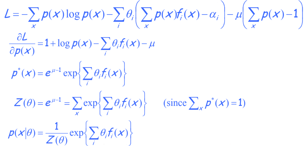
\[\sum_{x} p(x)f_i(x) = \alpha_i\]Assuming these expectations are consistent (ie we don’t say that the mean is both 1 and 2), there may exist many distributions that satisfy this constraint. We should select the most uncertain one. The one where the entropy $E[-log(p(x))]$ is maximized.
With this constraints, we can derive a simple optimization problem:
Using these constraints we can derive the best solution to this optimization problem:
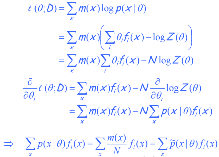
We have shown that assuming the distribution maximizes the entropy while matching some empirical feature averages forces the optimal solution to be in the exponential family. Interestingly, we can also prove this in the other direction.
Assuming that our solution is the MLE solution in the exponential family, we can derive that it will match empirical feature average
Conditional Random Fields (CRFs)
In this section, we will first motivate CRFs and discuss how they overcome the shortcomings of HMMs. Second, we will briefly describe its inference and learning mechanism. Next, we will mention some of its applications, and empirical successes. Lastly, we will conclude with some of the recent research on hybrid neural-CRFs.
Introduction
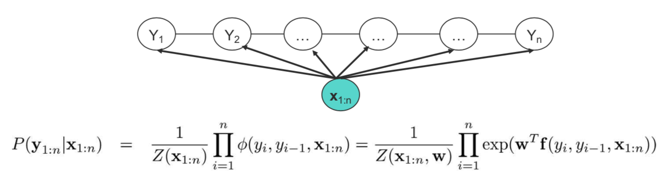
The graphical representation of a 1-D chain CRF is depicted in the figure above. CRFs can be thought of as an evolution of HMMs, but unlike HMMs they are discriminative models, and directly model the conditional distribution $P(\mathbf{Y}|\mathbf{X})$ instead of the joint distribution $P(\mathbf{X}, \mathbf{Y})$. Most often, we care about the prediction anyway, so modeling it directly avoids the computation of the joint probability.
CRFs offer two key advantages over HMMs:
- They model the entire observed sequence. For example, in a task where we want to predict the Part-Of-Speech (POS) tags for a sequence of words in a sentence, it helps to know the entire sequence of words while predicting the POS tag at time step $t$.
- They do not suffer from the label bias problem. We briefly discuss the problem below.
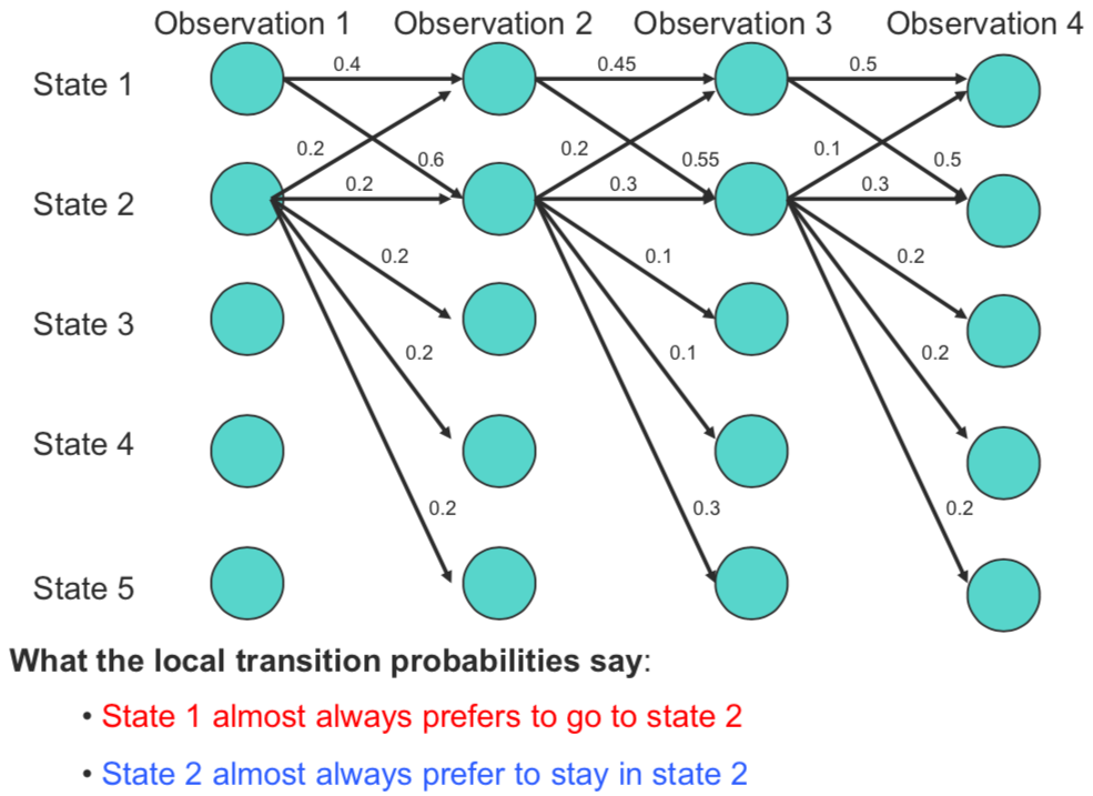
The Label Bias Problem:
In the figure above, we can observe that state 1 transitions into only two states (state 1, and 2); whereas state 2 can potentially transition into all the five available states. Furthermore, we observe that at every time step, state 1 always prefers to transition to state 2 over state 1, and similarly state 2 always prefers to transition to state 2 over other 4 options. However, path 1 -> 1 -> 1 -> 1 is the most likely path with probability of $0.09$, whereas the intuitively correct path of 1 -> 2 -> 2 -> 2 has a probability mass of only $0.054$. The reason for this counter-intuitive phenomena is rooted in the fact that probability mass from state 2 is distributed across all states. Thus, the probabilities being locally normalized is not desirable here. CRFs overcome this problem by having potential scores instead of probabilities, which are globally normalized.
Having motivated why such models might be useful, let us see to learn and do inference over these models.
Inference and learning
The inference algorithm for CRFs is very simple, and just like HMMs, we can do Viterbi decoding.
The task of learning is essentially learning the weights ($\mathbf{w}$) for the features $\mathbf{f}(y_i, y_{i-1}, \mathbf{x}_{1:n})$ used to score the configurations. One can draw parallels here to a well known class of discriminative classifiers — logistic regression, and just like logistic regression, we can do gradient ascent over the weights to increase the conditional probability over the observed set of $\mathbf{X}, \mathbf{Y}$ pairs. Given the 1-D chain structure, the normalizing term (or the partition function) can be tractably computed. In practice, gradient ascent has very slow convergence, and other alternatives like conjugate gradient method and limited memory quasi-newton methods can be used for faster learning. Most CRFs, especially ones involving arbitrary structure, are intractable in general owing to the difficulty in computing the partition function.
Applications: CRFs have been very successful in a wide range of applications across different fields. In NLP, they are commonly used for POS-tagging, Named Entity Recognition (NER), and other tagging problems. In computer vision, they have found utility in image segmentation, image restoration, handwriting recognition among other tasks.
Recent developments: A popular recent trend in NLP tagging problems is to combine CRFs with neural representations from CNNs, and LSTMs instead of the hand-crafted features $\mathbf{f}(y_i, y_{i-1}, \mathbf{x}_{1:n})$, and the weights for the CNNs and LSTMs are also learnt as a part of the learning process (through back-propagation).
Lastly, a tutorial