Lecture 8: Causal Discovery and Inference
Learning and inference algorithms for causal discovery.
Causation implies correlation (or dependence), but correlation does not imply causation. For example, consider the case of chocolate consumption vs. the number of Nobel Laureates in the country:
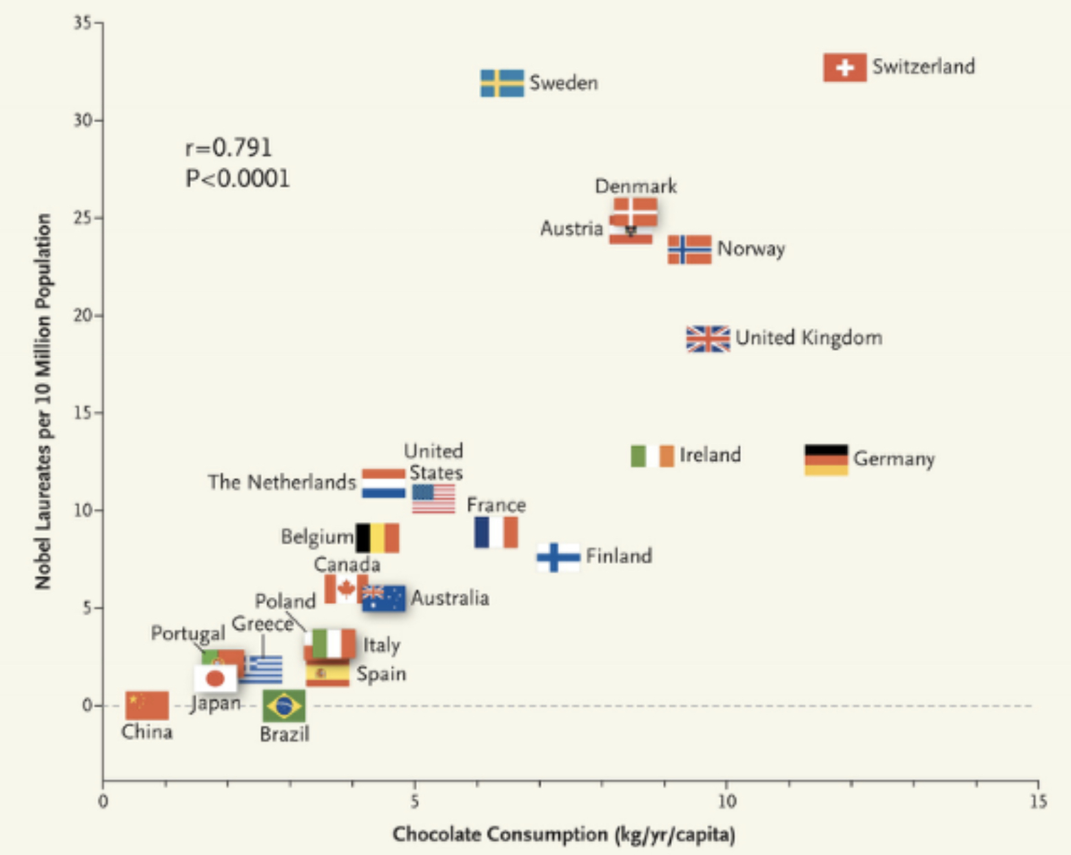
From this plot, we can see that they are highly correlated. But it is absurd to say that if we want to increase the number of Nobel Laureates in a country, we need to eat more chocolate. This is where the idea of causality comes in. They are correlated, but chocolate consumption is not the cause of Nobel Laureates. The following equations capture this difference mathematically:
$X$ and $Y$ are dependent if and only if $ \exists x_1 $ different than $ x_2 $ such that:
\[P(Y \mid X=x_{1}) \text{ different than } P(Y \mid X=x_2)\]$X$ is a cause of $Y$ if and only if $ \exists x_1 $ different than $ x_2 $ such that:
\[P(Y \mid do(X=x_1) \text{ different than } P(Y \mid X=x_2)\]The definition requires just a single pair of distinct $ x_1, x_2 $ to have different conditional distributions of $Y$. $Y$ may have the same conditional distribution over a range of $X$ values, but if we find even a single pair for which the conditional distribution is different, $X$ and $Y$ are dependent. The same goes for causation.
The causation definition is circular in the sense that, if we don’t know the causal relation of the other variables, we can’t define the intervention of $X$ and thus can’t find the causal relation of $X$ and $Y$. So in order to define one causal relation, we need all other causal relations.
Causal Thinking
Simpson’s Paradox
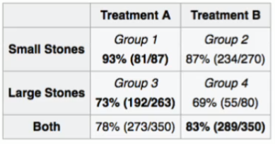
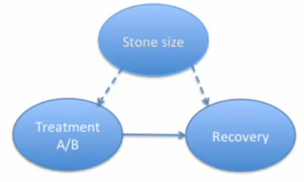
Example 1: Suppose there are two types of patients, one with small kidney stones and the other with large kidney stones. There are two types of treatments to choose from, A and B. From the data we can see that, if we consider the patient categories separately, treatment A has a higher recovery rate in both cases. But if we combine the categories of patients, we see that the treatment B has a higher recovery rate 83% (289/350). So, as a doctor, which treatment would you suggest to a patient?
Example 2: We plot cholesterol levels vs. the amount of exercise for people of different age groups. For each age group, we see that the more you exercise, the less cholesterol you have. But if we combine all the plots (of different age groups), we see the opposite result: the more you exercise, the more cholesterol you have.
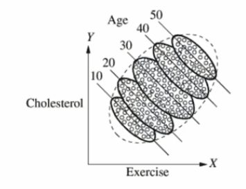
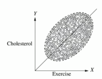
In both examples, there was a common cause between the quantities we were comparing, and due to this common cause, the relationship between the quantities can be arbitrary. We should fix the value of the common cause, and then see the relation between the quantities we want to compare.
Strange Dependence
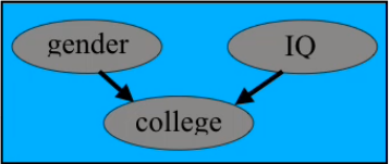
Example: If we go back 50 years, we observe that female college students score higher on IQ tests than male students on average. Gender and IQ are two very different quantities, and we can safely assume that they are independent. But given a common cause, like say going to college, now they become dependent. A simple way to understand this is as follows: Two independent variables $X$ and $Y$ become dependent if we condition on the sum of $X$ and $Y$.
Monty Hall problem
The setup is as follows. There are 3 doors, behind one of which there is $1000. If we select that door, we get the prize money. So we make our initial guess, then the game show host opens one of the empty doors and shows there is no money behind that door. Should we stick with our initial choice or switch to the other door?
The answer is to switch our choice. If we switch, our probabilty of winning becomes 2/3 rather than the 1/3 if we stick to our choice. We can think of it as follows. There are three options to select from initially, two empty doors and one with the prize money. If we are always switching, we will end up with the prize money if we have initially chosen the empty door and we will lose if we have initially selected the door with the prize money. So to win, we need to select the empty door at first whose probability is 2/3. So the chance of us winning the car if we switch is 2/3.
Causal Models
If we have causal models, it is very easy to do intervention. We just need to delete all the incoming edges into the nodes which we are intervening and then do inference on the obtained graphical structure.
Also if we know the causal structure, we can apply some of the known distributions into new scenarios. This idea is used in transfer learning.
Prediction
This answers the question of $ P(Y \mid X) $ which means the probability of $Y$ if $X$ happens to take a particular value. This can be found out just from the observational data. We don’t need any graphs, or causal realtions to find this value.
Intervention
This answers the question of $ P(Y \mid do(X)) $ which means what is the probability of $Y$ if $X$ is set to a particular value keeping all the other variables same. For this, we definitely need to know all the causal relations of all the variables.
Counterfactual Thinking
This answers the question of $ P(y_x \mid x’, y’) $, which is the probability that event $Y$ = $Y$ would be observed had $X$ been x, given that we actually observed $X$ to be $ x’ $ and and $Y$ to be $ y’ $. For this, again we require causal relations via the structural equation model.
Identification of Causal Relation
Causal DAGs
Each edge in a causal DAG corresponds to direct causal influence between the nodes and it is asymmetric. Let $ P_x(V) $ be the distribution resulting from intervention $ do(X=x) $. Then a DAG is a causal DAG if
-
$ P_x(V) $ is Markov relative to G. This distribution is still factorizable according to the Markov property (product of proabbility of each node given its parents) with respect to G
-
$ P_x(V_i = v_i) = 1 $ for $ V_i \in $X$ $ and $ v_i $ consistent with X=x. This is so because we have performed intervention on $X$ and we have set that to $X$. Hence we know those variables with absolute certainty.
-
$ P_x(V_i \mid PA_i) = P(V_i \mid PA_i) $ for all $ V_i \notin $X$ $ where $ PA_i $ represents the parents of $ V_i $. That means the conditional distributions of all the nodes not included in the intervention remains the same before and after the intervention. We can see this graphically since while doing intervention, we just delete all the incoming edges into the nodes on which intervention is performed. So the other nodes remain unchanges(in terms of parents)
Randomized Control Experiments
We change a controlled variable and observe the change in an outcome variable. All the other variables that influence the outcome variable is either fixed or varied at random. So now any change observed in the outcome variable must have been due to the change in the controlled variable.
Its disadvantage is that its expensive and in many cases impossible to do. The outcome variable can depend on many other variables. So, to find one causal relation, we would need a lot of data and we need to ensure that the other variables are fixed or varied randomly across the experiments which is a very hard task.
Kidney Stone Experiment
Let’s revisit the kidney stone treatment example. Let R = Recovery, T = Treatment and S = Stone size, then
\[P(R \mid T) = \sum_S P(R \mid S,T)P(S \mid T)\] \[P(R \mid do(T)) = \sum_S P(R \mid S,T)P(S)\]Note that while intervening, we cut off all incoming edges into the treatment node. So, now S and T are independent.
Causal Effect Identifiability
An aspect of a statistical model is identifiable, if it cannot be changed without there also being some change in the distribution of the observed variables. So if we can express a quantity as a function of the distributions of observed variables, then we can say that quantity is identifiable. Thus the causal effect is identifiable if and only if we can represent $ P(Y \mid do(X)) $ in terms of the distribution of observed variables. i.e. if
$ P_{M1}(Y \mid do(X)) = P_{M2}(Y \mid do(X)) $ for every pair of models M1 and M2 with the dame graph and the same distibution of observed variables(Unobserved / Latent variable distributions can be changed)
Example - If we have just two random variables $X$ and Y(both observed) where $X$ is the cause of $Y$ and there is no confounder.So, $ P(Y \mid do(X)) = P(Y \mid X) $ and we know this is identifiable because for changing $ P(Y \mid X) $, we would have to change the distribution of P(X,Y).
But, now lets say we have a confounder C, which is the common cause of both $X$ and $Y$. And this is not observed. Now, we can change the distribution of C such that P(X,Y) is unchanged but we get different $ P(Y \mid do(X)) $ $ P(Y \mid do(X)) $ can also be written as $ P(y \mid \hat{x}) $
Back-Door Criterion
A set of variables $Z$ satisfies the back-door criterion relative to an ordered pair of variables $(X_i, X_j)$ if
- No node in $Z$ is a descendant of $X_i$
- $Z$ blocks every path between $X_i$ and $ X_j $ that contains an arrow into $X_i$ (Hence the name back-door)
If the set of nodes $Z$ follows these two conditions then $ P (y \mid \hat{x}) = \sum_z P(y \mid x,z)P(z) $ Same as we saw earlier in the case of kidney stone treatment. And thus $ P(y \mid \hat{x}) $ is now identifiable because of this back-door adjustment.
Front-Door Criterion
A set of variables $Z$ satisfies the front-door criterion relative to an ordered pair of variables $(X_i, X_j)$ if
- $Z$ intercept all directed paths from $X$ to $Y$ (hence the name front-door)
- There is no back-door path from $X$ to $Z$
- All back-door paths from $Z$ to $Y$ are blocked by X If the set of nodes $Z$ follows these two conditions then
Unification
A sufficient condition under which the causal effect $ P(y \mid do(x)) $ is identifiable is that there exist no bi-directed path between $X$ and any of its children. For more information, this is presented in the paper “A General Identification Condition for Causal Effect”.
Propensity Score
The Average Causal Effect (ACE), defined as:
\[\mathbb{E} \left[ $Y$ \mid do(x) \right] - \mathbb{E} \left[ $Y$ \mid do(x') \right]\]Given that $ P(Y \mid do(x)) = \sum_{c} P(Y \mid x,c)P(c) $ might not share the same $ P(c) $, one solution for an estimator of the ACE can be through direct matching. If $ C $ is a high dimensional space one can use the propensity score to achieve unconfoundedness and estimate ACE.
Causal Discovery
Causal discovery relies on two assumptions:
-
Causal Markov condition: Each variable is independent of its non-descendants given its parents.
-
Faithfulness condition: All observed (conditional) independencies are captured in the causal graph. Roughly speaking, faithfulness allows you to go back from independence to causal graph.
The above two conditions allows us to determine a list of candidate causal structures, with the same causal skeleton. Following this, we need to determine the causal direction. This step involves finding v-structure and doing orientation propagation.
The following example as given in lecture for reasoning about independence conditions:
Suppose you have four variables $ X_1, X_2, X_3, X_4 $ such that: \(X_1 \perp X_2\)
\[X_1 \perp X_4 \mid X_3\] \[X_2 \perp X_4 \mid X_3\]The question is: can there exist a confounder behind $X_3$ and $X_4$?
The answer is no. As if there is a confounder C which is the parent of both $ X_3 $ and $ X_4 $, then the path between $ X_1, X_3, C, X_4 $ is open, thus $ X_1 \not\perp X_4 \mid X_3 $.
This is one example where the independence conditions allow us to reason about the structure of the graph.
Nevertheless, this does not mean we can always determine the graph as two DAGs may have the same skeleton and v-structure. We can sometimes only recover graphs of the same equivalence class.
Constraint-Based Causal Discovery
Constraint-Based Causal Discovery makes use of conditional independence constraints. It relies on causal Markov condition + faithfulness assumption.
Remember,
Causal Markov condition: each variable is independent of its non-descendants (non-effects) conditional on its parents (direct causes)
Faithfulness: all observed (conditional) independencies are entailed by Markov condition in the causal graph
(Conditional) independence constraints give us candidate causal structures. Discovery is done using the PC Algorithm.
PC Algorithm
This algorithm relies on markov assumption and faithfulness assumption. Moreover, it relies on the key idea that if $ (X, Y) $ not adjacent then $X$ and $Y$ are d-separated either given pa(X) or pa(Y ):
Then the algorithm involves:
- For each pair (X, Y), test $ $X$ \perp $Y$ \mid \varnothing $, if the independence holds, remove the edge.
- For each pair (X,Y) adjacent, with $ \text{max} \mid Adj(X) \mid, \mid Adj(Y) \mid \geq 2 $, test $ $X$ \perp $Y$ \mid S $ where $ \mid S \mid = 1 $ and $ S \subseteq Adj(X) $ or $ S \subseteq Adj(Y) $.
- …
- For each pair (X,Y) adjacent, with $ \text{max} \mid Adj(X) \mid, \mid Adj(Y) \mid \geq k+1 $, test $ $X$ \perp $Y$ \mid S $ where $ \mid S \mid = k $ and $ S \subseteq Adj(X) $ or $ S \subseteq Adj(Y) $.
We stop when we reach k s.t for all (X,Y), $ \text{max} \mid Adj(X) \mid, \mid Adj(Y) \mid < k+1 $ (since it’s enough to find one set of nodes that make $X$ and $Y$ independent to remove their edge).