Lecture 9: Modeling Networks
Classic network learning algorithms.
Network research - study at graph as object
How do we estimate graphs given real-world data? Different generation rules will produce different graphs. We explore such methods here.
Structural Learning
Trees: The Chow-Liu algorithm
The Chow-Liu algorithm directly searches for the optimal tree structure.
Pairwise Markov Random Fields
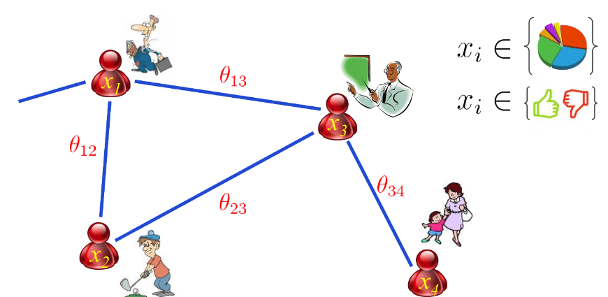
The key idea for graph structure learning is that we should view network inference as parameter estimation. Every node in the graph can be either binary or continuous number. All the variables are connected pairwise, which gives us pairwise Markov Random Field, also Boltzmann Machine. The joint probability of all the nodes is represented as
\[p(x_1, x_2, x_3, x_4) = \frac{1}{Z} exp\{\theta_1x_1 + \theta_2x_2 + \theta_3x_3 + \theta_4x_4 + \theta_{12}x_1x_2 + \theta_{13}x_1x_3 + \theta_{23}x_2x_3 + \theta_{34}x_3x_4 \}\]we use non-zero parameters to represent the existence of edges. This equivalence is prominent because we turn topology into continuous space.
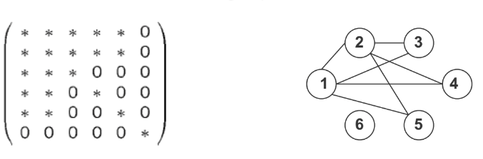
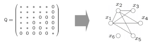
Structure of many classic models can be learned by this algorithm. For discrete node states, we have the Ising/Potts model; for continuous nodes, we have the Gaussian graphical model; finally, we can also have the heterogeneous model with both discrete and continuous nodes. The key take away is parameter matrix encodes graph structure (non zero $\iff$ edge)
Multivariant Gaussian
Recall the definition of multivariant Gaussian
\[p(\vec x \mid \mu, \Sigma) = \frac{1}{(2\pi)^{\frac{n}{2}}|\Sigma|^{\frac{1}{2}}} exp\{-\frac{1}{2}(\vec x - \mu)^T \Sigma^{-1} (\vec x - \mu) \}\]Let $\mu = 0, Q = \Sigma^{-1}$, we have
\[p(x_1,x_2,...,x_p|\mu = 0,Q) = \frac{|Q|^\frac{1}{2}}{(2\pi)^{\frac{n}{2}}} exp \{ -\frac{1}{2} \sum_{i}q_{ii}(x_i)^2 - \sum_{i < j} q_{ij}x_ix_j \}\]This equation can be viewed as a continuous Markov Random Field with potentials defined on every node and edge. $q_{ii}(x_i)^2$ can be treated as the node potential, while $q_{ij}x_ix_j$ can be treated as the edge potential.
Gaussian Graphical Model
Consider the model on a zero-mean Gaussian distribution \(\textbf{X}^{(n)} \sim \mathcal{N}(\textbf{0}, \Sigma^{(n)})\)
where $\Sigma^{(n)}$ encode dependencies among variables. As we mentioned before, the inverted matrix of the covariance matrix is called the precision matrix which encodes non-zero edges in Gaussian Graphical Model.
Markov vs Correlation Network
While these two models have their similarity, Markov fits more on the real world because it can model conditional probabilities.
Correlation network
\[\Sigma_{i,j} = 0 \Rightarrow X_i \perp X_j \quad or \quad p(X_i, X_j) = p(X_i)p(X_j)\]Correlation network is based on covariance matrix $\Sigma$. So $\Sigma_{i,j} = 0$ means that $X_i$ and $X_j$ are marginally independent without observing other variables. In fact, this kind of independence is hard to find in the real world problems
Gaussian Graphical Model
\[Q_{i,j}=0 \Rightarrow X_i \perp X_j \mid X_{-ij} \quad or \quad p(X_i, X_j \mid X_{-ij}) = p(X_i \mid X_{-ij})p(X_j \perp X_{-ij})\]A Gaussian Graphical Model (GGM) is a Markov Network based on precision matrix $Q$. Compared with independencies in Correlation network, conditional independence/partial correlation coefficients are more sophisticated dependence measures. This kind of independence is more suitable for modeling real-world situations.
However, there are still noticeable problems with learning the dependencies of Gaussian Graphical Model. First, the algorithm wants the precision matrix to be invertible, but non-full rank does not mean MN does not exist. Also, with a small sample size, empirical covariance matrix cannot be inverted. Second, the computational complexity of inverting a matrix is $O(N^3)$ where N is the number of node in a graph. Last but not least, inversion of the matrix is not scalable to high dimensions.
Now that our purpose is to obtain the precision matrix, so we need to make an assumption to avoid these problems.
Prior Assumption of GGM - Sparsity
We make a common assumption that the precision matrix $Q$ is sparse in real problems. This assumption makes empirical sense because, for example, Genes are only assumed to interface with a small group of other genes. It also makes statistical sense as learning is feasible in high dimensions with small sample.
After making this assumption, it is still hard to get the whole precision matrix. What if we get the precision matrix row by row or column by column. Then it came to the basic method to make this simpler thought possible.
GGM with Lasso
Our target is to select the neighborhood of each node so we can perform regression of all nodes to express the relationship between two nodes according to the parameters in the regression. However, there will be a problem that as long as we use the normal regression to one node, other nodes in the network would be the neighborhood of this node since the parameters are non-zero. That is the reason why we need LASSO regression, which can cause zero parameters through penalty. Therefore, the regression problem at each node can be formulated the following LASSO problem:
\[\hat{\beta_{1}} = \arg\min_{\beta_{1}} \|\textbf{Y} - \textbf{X}\beta_{1}\|^{2} + \lambda\|\beta_{1}\|_{1}\]where $\textbf{Y}$ is an N dimensional vector with each entry being a node at a specific dimension from the N sets of data observations. Each set of data observation has P nodes, which is illustrated as the P nodes forming a circle in the following figures.
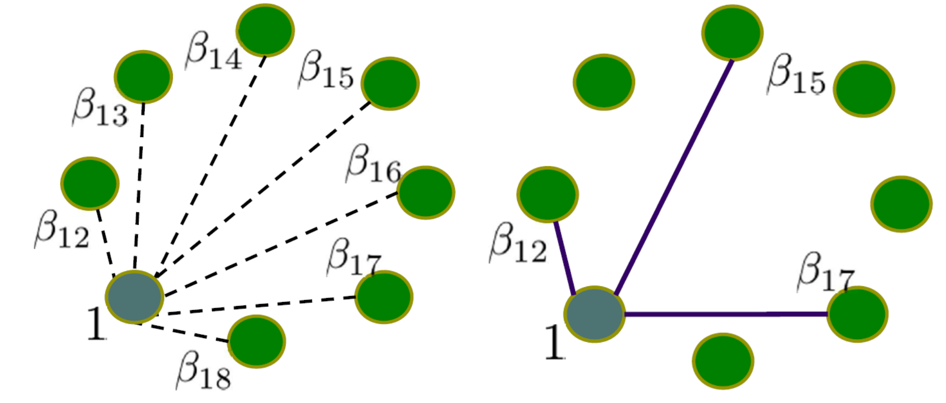
$\textbf{X}$ is an $N \times (P −1)$ dimensional matrix with each column being the rest of the nodes in the N sets of observations. $\beta_1$ is a P − 1 dimensional coefficient weight vector one wants to estimate. The last $l_1$ term in the equation is the sparse promoting penalty term that enforces sparsity. Notice ideally we want to use $| \beta_1 |_{0}$ which is the $l_0$ term to minimize the number of supports. However this makes the problem non-convex and difficult to solve. One therefore relaxes this problem to the $l_1$ case. The above regression is repeated for each node and the zero valued edges are removed. Generally, one is more interested in whether pairwise nodes are conditionally independent or not.
Only when the following assumptions are met, LASSO regression can asymptotically recover correct subset of covariates that relevant.
- Dependency Condition: Relevant Covariates are not overly dependent
- Incoherence Condition: Large number of irrelevant covariates cannot be too correlated with relevant covariates
- Strong concentration bounds: Sample quantities converge to expected values quickly
And theoretically, there is a proof that graphical lasso can recover the true structure of the graph
then with high possibility,
\[S(\hat{\beta}) \to S(\beta_{\ast})\]Why does this algorithm work?
After knowing the process of this algorithm to obtain the precision matrix through repeatedly applying LASSO regression on each node, we want to know why we can get the precision matrix in this way. In other words, we want to know why LASSO regression can select the neighborhood of each node.
Multivariate Gaussian
For the multivatiate Gaussian there are several formulas to remember
\[p(x_2) = \mathcal{N}(x_2 | \mu_2, \Sigma_{22})\] \[p(x_1|x_2) = \mathcal{N}(x_1 | \mu_{1|2}, V_{1|2})\]where we have $ \mu_{1|2} = \mu_1 + \Sigma_{12}\Sigma_{22}^{-1}(x_2 - \mu_2) $ and $ V_{1|2} = \Sigma_{11} - \Sigma_{12}\Sigma_{22}^{-1}\Sigma_{21} $
The matrix inverse lemma
Consider a block-partitioned matrix:
\[M= \left[ \begin{matrix} E & F \\ G & H \\ \end{matrix} \right]\]We diagonalize $M$ firstly
\[\left[ \begin{matrix} I & -FH^{-1} \\ 0 & I \\ \end{matrix} \right] \left[ \begin{matrix} I & 0 \\ G & H \\ \end{matrix} \right] \left[ \begin{matrix} I & 0 \\ -H^{-1}G & I \\ \end{matrix} \right] = \left[ \begin{matrix} E-FH^{-1}G & 0 \\ 0 & H \\ \end{matrix} \right]\]According to the Schur complement $M/H = E-FH^{-1}G$ , then we use this formula $XYZ = W \Rightarrow Y^{-1} = ZW^{-1}X$ to inverse
The matrix inverse lemma is
\[(E-FH^{-1}G)^{-1} = E^{-1} +E^{-1}F(H-GE^{-1}F)^{-1}GE^{-1}\]The covariance and the precision matrices
If we have the covariance matrix
\[\Sigma= \left[ \begin{matrix} \sigma_{11} & \vec{\sigma}_1^{T} \\ \vec {\sigma}_1 & \Sigma_{-1} \\ \end{matrix} \right]\]Also recall the facts about matrix inverse derived in the previous section, we can have the precision matrix:
\[Q= \left[ \begin{matrix} q_{11} & -q_{11}\vec{\sigma}_1^{T}\Sigma_{-1}^{-1} \\ -q_11\Sigma_{-1}^{-1}\vec {\sigma}_1 & \Sigma_{-1}^{-1}(I+q_{11}\vec {\sigma}_1\vec{\sigma}_1^{T}) \\ \end{matrix} \right] = \left[ \begin{matrix} q_{11} & \vec q_1^T \\ \vec q_1& Q_{-1} \\ \end{matrix} \right]\]Justification
With the above three facts, one is ready to justify why the problem can be formulated as a LASSO variable selection problem. Given a Gaussian distribution, the conditional distribution of a single node i given the rest of the nodes can be written as:
\[p(X_i|\textbf{X}_{-i}) = \mathcal{N}(\mu_i+\Sigma_{X_i\textbf{X}_{-i}}\Sigma_{\textbf{X}_{-i}\textbf{X}_{-i}}^{-1}(\textbf{X}_{-i}-\mu_{\textbf{X}_{-i}}),\Sigma_{X_iX_i} - \Sigma_{X_i\textbf{X}_{-i}}\Sigma_{\textbf{X}_{-i}\textbf{X}_{-i}}^{-1}\Sigma_{\textbf{X}_{-i}X_i})\]Let $\mu = 0$ we have
\[p(X_i|\textbf{X}_{-i}) = \mathcal{N}(\frac{\vec q_i}{-q_{ii}}\textbf{X}_{-i}, q_{i|-i})\]From here we can already see that the value of a certain node is determined by the linear representation of the other nodes plus a Gaussian noise:
\[X_i \gets \beta_i\textbf{X}_{-i}+Noise(Gaussian)\]Neighborhood estimation based on auto-regression coeficient
\[S_i \equiv \{ j:j \not = i, \theta_{ij} \not = 0\}\]If we are given the estimation of the neighborhood $S_i$ we have
\[p(X_i|\textbf{X}_{-i}) = p(X_i|\textbf{X}_{S})\]Therefore, the neighborhood $S_i$ defines the Markov blanket of node $i$ . That is the reason why we can use LASSO regression to each node in order to get the precision matrix.
Discrete Models
Given vector $\mathbf{x}$, how do we find the structure $s_x$? We just showed that this can be done via regression. %We can start by estimating $Q = \Sigma^{-1}$ What if we assume that nodes are discrete? Let’s assume that the edges. Then for a given sample x:
\[P(x | \Theta) = exp ( \sum_{i \in V} \theta^t_{ii}x_i + \sum_{(i, j) \in E} \theta_{ij} x_i x_j - A(\Theta) )\]If our observation are discrete, we can still estimate a graph in the same spirit as in the continuous case shown above. However, we can not do linear regression in the discrete case. So instead we will employ logistic regression. Namely,
\[P_\theta(x_k | x_{\setminus k}) = \text{ logistic }(2x_k\langle \theta_{\setminus k}, x_{\setminus k} \rangle)\]We can now apply similar techniques to those shown above, but with this new loss function. Implicitly, we assume, as we did before, that each observation $x_k$ is a scalar. What if we were in the case where $x_k$ is a vector? Or in the case where $x_k$ is a vector, but $x_i$ (where $i \neq k$) is a vector of a different dimensionality? Our standard linear regression ($y = \beta x + \sigma$ from above), or our logistic regression, assume that our observations are scalars. Instead of estimating the regression coefficients, we instead estimate the partial correlation. This details of this approach goes beyond the scope of this lecture.
Evolving Networks
Networks are not always constant across time. Let’s assume that you have data from varying time points. It may not be a reasonable assumption that each data point is generated from the same network. Now, a reasonable question to ask is, “At some given time T, what would our network be”? This violates our independent and identically distributed ($i.i.d$) assumption that we often make. To complicate matters further, at time T, we may have only one data point (or a small number of data points) to work with.
We introduce the Kernel Weighted $L_1$-regularized Logistic Regression:
\[\hat{\theta_i^t} = \arg\min_{\theta_i^t} l_w(\theta_i^t) + \lambda_1||\theta_i^t||_1 \forall t\]such that:
\[l_w(\theta_i^t) = \sum_{t' = 1}^T w(x^{t'}; x^t)\log(P(x_i^{t'}| \mathbf{x}_i^{t'}, \theta_i^t))\]Here, we are assuming that we still have the full data set. We weight each datapoint based on it’s relationship to our current time. For example, points that are closer to our time point T are weighted more than time points further away. Specifically, we can assume that data taken closer to time point T are more reflective of our graph at time T that points sampled at a more distant time. We can think of this weight as saying “how much do I trust this data point to inform about the graph at time point T”. The selection of these weights is typically done using a kernel (e.g. a gaussian kernel). Now we can use our T data points to estimate T graphs instead of a single graph. It can be shown that this method has the same consistency as if we had used i.i.d data with a few reasonable assumptions, such that our graph changes smoothly across time.
While not directly covered, in lecture, the Temporally Smoothed $L_1$-regularized Logistic Regression (TESLA) is another method for computing graphs across time. Specifically:
\[\hat{\theta}_i^1,...,\hat{\theta}_i^T = \underset{\hat{\theta}_i^1,...,\hat{\theta}_i^T}{\text{argmin}} \sum_{t=1}^T l_{avg}(\theta_i^t) + \lambda_1 \sum_{t=1}^T ||\theta^t_{-1} ||_1 + \lambda_2 \sum_{t=2}^T ||\theta^t_{-1} - \theta^{t-1}_{-1}||_q^q\]such that
\[l_{avg}(\theta_i^t) = \frac{1}{N^t} \sum_{d=1}^{N^t} \log(P(x_{d, i}^t | \mathbf{x}^t_{d, -i}, \theta^t_i))\]This is equivlent to solving the following constrained optimization problem:
This algorithm serves as an extension of the temporally smoothed $l_1$-regularized logistic regression algorithm (TESLLOR). Like KELLER, there is also the assumption that networks that are closer together in time are more likely to be similar to each other. TESLA, however, can handle abrupt changes across time. For more information, see