Lecture 10: Sequential Models

Introducing State Space Models and Kalman filters.

Mixture Models Review and Intuition to State Space Models

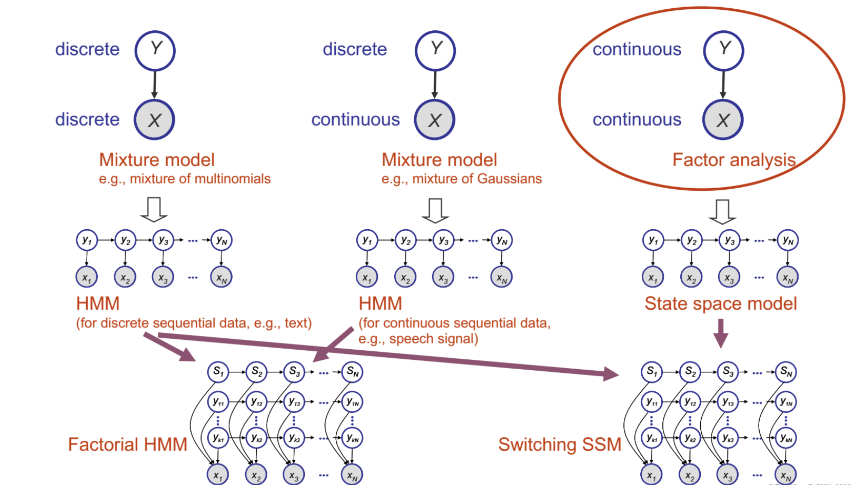
**Review and intuition of HMMs and SSMs**

Mixture model has the observation X and their corresponding hidden latent variable Y which indicates the source of that observation X. Observation X can be discrete like word frequency, or continuous like temperature. Variable Y denotes which mixture/distribution X comes from. When both X and Y are continuous, it is called factor analysis.
The advantage with mixture models is that smaller graphs (mixture models) can be taken as building blocks to make bigger graphs (HMMs)
Some common inference algorithms for HMMs can range from inferring on one hidden state, all hidden states, and even the most probable sequence of hidden states. Example algorithms are Viterbi algorithm, Forward/Backward algorithm, Baum-Welch algorithm.
All the above algorithms have a counterpart in State Space models - despite the mathematical technique being different, they have the same essence. A similarity to the above algorithms that it shares is that it can be broken down into local operations/subproblems and continuously built to the whole solution. We will further explain in the coming sections.
Stories/Intuitions for the various models

HMM - Dishonest casino story
Factorial HMM - Multiple dealers at the dishonest casino
State Space Model (SSM) - X – Signal of an aircraft on the radar, Y – actual physical locations of the aircraft
Switching SSM - multiple aircrafts (State S is the indicator of which aircraft is appearing on the radar)

Basic Math Review

A multivariate Gaussian is denoted by the following PDF -

P(X | \mu, \Sigma) = \frac{1}{(2\pi)^{n/2} |\Sigma|^{1/2}} \exp(\frac{-1}{2}(X - \mu)^{T}\Sigma^{-1}(X-\mu))

A Joint Gaussian is denoted by -

P(\begin{bmatrix} X_1 \\ X_2 \end{bmatrix} | \mu, \Sigma) = \mathcal{N}(\begin{bmatrix} X_1 \\ X_2 \end{bmatrix} | \begin{bmatrix} \mu_1 \\ \mu_2 \end{bmatrix}, \begin{bmatrix} \Sigma_{11} & \Sigma_{12} \\ \Sigma_{21} & \Sigma_{22} \end{bmatrix})

Given the joint distribution, we can write -

\begin{aligned} &P(X_2) = \mathcal{N}(X_2 | \mu_2, \Sigma_{22}) \\ &P(X_1 | X_2) = \mathcal{N}(X_1 | \mu_{1|2}, V_{1|2}) \\ &\mu_{1|2} = \mu_1 + \Sigma_{12}\Sigma_{22}^{-1}(X_2 - \mu_2) \\ &V_{1|2} = \Sigma_{11} - \Sigma_{12}\Sigma_{22}^{-1}\Sigma_{21} \end{aligned}

Matrix inverse lemma -

Consider a block partitioned matrix M = \begin{bmatrix} E & F \\ G & H \end{bmatrix}
First we diagonalize M - \begin{bmatrix} I & -FH^{-1} \\ 0 & I \end{bmatrix}\begin{bmatrix} E & F \\ G & H \end{bmatrix}\begin{bmatrix} I & 0 \\ -H^{-1}G & I \end{bmatrix} = \begin{bmatrix} E-FH^{-1}G & 0 \\ 0 & H \end{bmatrix}
This is called the Schur's complement - M/H = E-FH^{-1}G
Then we inverse using the formula - \begin{aligned} XYZ = W \implies Y^{-1} = ZW^{-1}X \implies M^{-1} = \begin{bmatrix} E & F \\ G & H \end{bmatrix}^{-1} = \begin{bmatrix} I & 0 \\ -H^{-1}G & I \end{bmatrix}\begin{bmatrix} (M/H)^{-1} & 0 \\ 0 & H^{-1} \end{bmatrix}\begin{bmatrix} I & -FH^{-1} \\ 0 & I \end{bmatrix} \\ = \begin{bmatrix} (M/H)^{-1} & -(M/H)^{-1}FH^{-1} \\ -H^{-1}G(M/H)^{-1} & H^{-1} + H^{-1}G(M/H)^{-1}FH^{-1} \end{bmatrix} \\ = \begin{bmatrix} E^{-1} + E^{-1}F(M/E)^{-1}GE^{-1} & -E^{-1}F(M/E)^{-1} \\ -(M/E)^{-1}GE^{-1} & (M/E)^{-1} \end{bmatrix} \end{aligned}
Hence, by matrix inverse lemma, (E - FH^{-1}G)^{-1} = E^{-1}+ E^{-1}F(H-GE^{-1}F)^{-1}GE^{-1}

Review of Basic matrix algebra -

Trace - tr[A]^{def} = \Sigma_i a_{ii}
tr[ABC] = tr[CBA] = tr[BCA]
Derivatives - \begin{aligned} \frac{\partial}{\partial A}tr[BA] = B^{T} \\ \frac{\partial}{\partial A}tr[x^{T}Ax] = \frac{\partial}{\partial A}tr[xx^{T}A] = xx^{T} \end{aligned}
Derivates - \frac{\partial}{\partial A}log|A| = A^{-1}

Factor analysis

Imagine a point on a sheet of paper x \in \mathcal{R}^2 If the orientation or the axes are changed, it could be viewed as a point in 3D-space as well. Depending on whether one is sitting in the room or on the paper, we will see the point in 2D or 3D. Hence Y is what is observed from our view (room or on paper), and X (the original point) is what is the hidden/latent variable.

\begin{aligned} P(X) = \mathcal{N}(X;0, I) \\ P(Y | X) = \mathcal{N}(Y; \mu+\Lambda X, \Psi) \end{aligned}

**Factor analysis for a point on a paper**

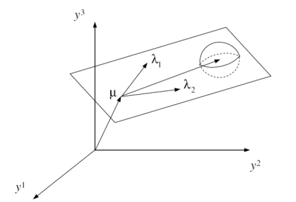
We know that, a marginal gaussian (p(X)) times a conditional gaussian (p(Y|X)) is a joint gaussian, and a marginal (p(Y)) of a joint gaussian (p(X, Y)) is also a gaussian. Hence, we can compute the mean and variance of Y. Assuming noise W is uncorrelated with the data,

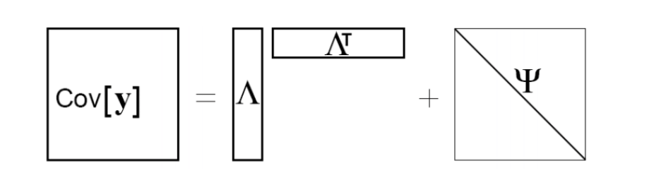
\begin{aligned} &W = \mathcal{N}(0, \Psi) \\ &E[Y] = E[\mu + \Lambda X + W] \\ & = \mu + 0 + 0 = \mu \\ &Var[Y] = E[(Y-\mu)(Y-\mu)^T] \\ & = E[(\mu + \Lambda X + w - \mu)(\mu + \Lambda X + w - \mu)^T] \\ & = E[(\Lambda X + w)(\Lambda X + w)^T] \\ & = \Lambda E[XX^T]\Lambda^T + E[WW^T] \\ & = \Lambda \Lambda^T + \Psi \end{aligned}

Hence, the marginal density for factor analysis (Y is p-dim, X is k-dim):

P(Y|\theta)= \mathcal{N}(Y;\mu, \Lambda \Lambda^T + \Psi)

We can also say, that the effective covariance matrix is a low-rank outer product of two long skinny matrices plus a diagonal matrix. In other words, factor analysis is just a constrained Gaussian model.

We will now analyse the Factor analysis joint distribution assuming noise is uncorrelated with the data or the latent variables - The distributions as we derived/assumed above are- \begin{aligned} &P(X) = \mathcal{N}(X;0, I) \\ &P(Y | X) = \mathcal{N}(Y; \mu+\Lambda X, \Psi) \end{aligned} The covariance between X and Y can be derived as follows - \begin{aligned} Cov[X, Y] = E[(X - 0)(Y - \mu)^T] = E[X(\mu + \Lambda X + W -\mu)^T] \\ = E[XX^T\Lambda^T + XW^T] = \Lambda^T \end{aligned} Hence the joint distribution of X and Y is - P(\begin{bmatrix} X \\ Y \end{bmatrix}) = \mathcal{N}(\begin{bmatrix} X \\ Y \end{bmatrix} | \begin{bmatrix} 0 \\ \mu \end{bmatrix}, \begin{bmatrix} I & \Lambda^T \\ \Lambda & \Lambda \Lambda^T + \Psi \end{bmatrix})

Now we can say - \begin{aligned} &\Sigma_{11} = I \\ &\Sigma_{12} = \Sigma_{21}^T = \Lambda^T \\ &\Sigma_{22} = \Lambda \Lambda^T + \Psi \end{aligned} Given all of the above, we can now derive the posterior of the latent variable X given Y, where \begin{aligned} &P(X|Y) = \mathcal{N}(X | \mu_{1|2}, V_{1|2}) \\ &\mu_{1|2} = \mu_1 + \Sigma_{12}\Sigma_{22}^{-1}(X_2 - \mu_2) \\ & = \Lambda^T(\Lambda\Lambda^T + \Psi)^{-1}(Y - \mu) \\ &V_{1|2} = \Sigma_{11} - \Sigma_{12}\Sigma_{22}^{-1}\Sigma_{21} = I - I\Lambda^T(\Lambda\Lambda^T + \Psi)^{-1}\Lambda I \end{aligned} Applying the matrix inversion lemma we learnt above, we get - \begin{aligned} &(E - FH^{-1}G)^{-1} = E^{-1}+ E^{-1}F(H-GE^{-1}F)^{-1}GE^{-1} \\ &V_{1|2} = (I + \Lambda^T\Psi^{-1}\Lambda)^{-1} \\ &\mu_{1|2} = V_{1|2}\Lambda^T\Psi^{-1}(Y-\mu) \end{aligned}

Learning in Factor Analysis

The inference problem, as shown above can be thought of as a linear projection since the posterior covariance ($V_{1|2}$ above) does not depend on the observed data $y$ and the posterior mean $\mu_{1|2}$ is just a linear operation.

The learning problem in Factor Analysis corresponds to learning the parameters of the model, i.e., the loading matrix $\Lambda$, manifold center $\mu$ and the diagonal covariance matrix of the noise, $\Psi$. As always, we will solve this problem by maximizing the log-likelihood of the observed data, i.e. $(\mu^*, \Lambda^*, \Psi^*) =$ argmax $\ell(\mathcal{D} ; \mu, \Lambda, \Psi)$.

Thanks to the derivation above, we have a closed-form expression for the incomplete log likelihood of the data, i.e. $\mathcal{D} = \text{\textbraceleft} y^{(i)} : i=1,…,n \text{\textbraceright} $, as shown below:

\begin{aligned} &\ell(\mathcal{D} ; \mu, \Lambda, \Psi) = \text{log} \; \Pi_{i=1}^{n} \frac {1} {(2 \pi)^{p} |\Lambda \Lambda^T + \Psi|^{1/2}} \text{exp} (-\frac{1}{2} (y^{(i)} - \mu)^T(\Lambda \Lambda^T + \Psi)(y^{(i)} - \mu)) \\ &= -\frac{n}{2} \text{log} (|\Lambda \Lambda^T + \Psi|) -\frac{1}{2} \sum_{i=1}^{n} (y^{(i)} - \mu)^T(\Lambda \Lambda^T + \Psi)(y^{(i)} - \mu) \\ &= -\frac{n}{2} \text{log} (|\Lambda \Lambda^T + \Psi|) -\frac{1}{2} tr[(\Lambda \Lambda^T + \Psi)^{-1}S] \; \\ & \text{where} \; S = \sum_{i=1}^{n} (y^{(i)} - \mu)(y^{(i)} - \mu)^T \end{aligned}

Estimation of $\mu$ is straightforward, however $\Lambda$ and $\Psi$ are tightly coupled non-linearly in log-likelihood. In order to make this problem tractable, we will use the same trick used in Gaussian Mixture Models, i.e., optimize the complete log-likelihood using Expectation Maximization (EM) algorithm.

\begin{aligned} &\ell_C(\mathcal{D} ; \mu, \Lambda, \Psi) = \sum_{i=1}^{n} \text{log} \; p(x^{(i)}, y^{(i)}) \\ &= \sum_{i=1}^{n} \text{log} \; p(x^{(i)}) \; \text{log} \; p(y^{(i)} | x^{(i)}) \\ &= -\frac{n}{2} \text{log} (|I|) - \frac{1}{2} \sum_{i=1}^{n} (x^{(i)})^T x^{(i)} + \\ & -\frac{n}{2} \text{log} (|\Psi|) - \frac{1}{2} \sum_{i=1}^{n} (y^{(i)} - \Lambda x^{(i)})^T (y^{(i)} - \Lambda x^{(i)}) \\ &= -\frac{n}{2} \text{log} (|\Psi|) - \frac{1}{2} \sum_{i=1}^{n} tr[(x^{(i)})^T x^{(i)}] -\frac{n}{2} tr[S\Psi^{-1}] \\ & \; \text{where} \; S = \frac{1}{n} \sum_{i=1}^{n} (y^{(i)} - \Lambda x^{(i)})(y^{(i)} - \Lambda x^{(i)})^T \end{aligned}

In the E-step of the EM procedure, we compute the expectation of the complete log-likelihood wrt the posterior, i.e., $p(x|y)$:

\begin{aligned} &\mathbb{E} [\ell_C(\mathcal{D} ; \mu, \Lambda, \Psi)] = -\frac{n}{2} \text{log} (|\Psi|) - \frac{1}{2} \sum_{i=1}^{n} tr[\mathbb{E} [(x^{(i)})^T x^{(i)} | y^{(i)}]] -\frac{n}{2} tr[\mathbb{E} [S | y^{(i)}]\Psi^{-1}] \\ & \text{where} \; \mathbb{E} [S] = \frac{1}{n} \sum_{i=1}^{n} (y^{(i)}(y^{(i)})^T - y^{(i)} \mathbb{E} [(x^{(i)})^T | y^{(i)}] \Lambda^T \\ & + \Lambda \mathbb{E} [(x^{(i)})^T | y^{(i)}] (y^{(i)})^T + \Lambda \mathbb{E} [(x^{(i)})^T x^{(i)} | y^{(i)}] \Lambda^T) \end{aligned}

Further, we use the posterior density calculations in the previous section to obtain the different expectations in the equation above:

\begin{aligned} &\mathbb{E} [x^{(i)} | y^{(i)}] = \mu_{1|2} \\ &\mathbb{E} [(x^{(i)})^T x^{(i)} | y^{(i)}] = Var[x^{(i)} | y^{(i)}] + \mathbb{E} [x^{(i)} | y^{(i)}] \mathbb{E} [x^{(i)} | y^{(i)}]^T \\ &= V_{1|2} + \mu_{1|2} \mu_{1|2}^T \end{aligned}

In the M-step, we take derivatives of the expected complete log-likelihood calculated above wrt the parameters and set them to zero. We shall use the trace and determinant derivative rules derived above in this step.

\begin{aligned} &\frac{\partial \ell_C}{\partial \Psi^{-1}} = \frac {n}{2} \Psi - \frac {n}{2} \mathbb{E} [S] \\ &\implies \Psi^{t+1} = \mathbb{E} [S] \end{aligned}

In a similar fashion,

\begin{aligned} &\frac{\partial \ell_C}{\partial \Lambda} = -\frac {n}{2} \Psi^{-1} \frac{\partial \mathbb{E} [S]}{\partial \Lambda} \\ &= \Psi^{-1} \big( \sum_{i=1}^{n} y^{(i)} \mathbb{E} [(x^{(i)})^T | y^{(i)}] - \Lambda \sum_{i=1}^{n} \mathbb{E} [(x^{(i)})^T x^{(i)} | y^{(i)}] \big) \\ &\implies \Lambda^{t+1} = \big(\sum_{i=1}^{n} y^{(i)} \mathbb{E} [(x^{(i)})^T | y^{(i)}] \big) \big( \sum_{i=1}^{n} \mathbb{E} [(x^{(i)})^T x^{(i)} | y^{(i)}] \big)^{-1} \end{aligned}

It should be noted that this model is “unidentifiable” in the sense that different runs for learning parameters for the same dataset are not guaranteed to obtain the same solution. This is because there is degeneracy in the model, since $\Lambda$ only occurs in the product of the form $\Lambda \Lambda^T$, making the model invariant to rotations and axis flips in the latent space. To see this more clearly, if we replace $\Lambda$ by $\Lambda Q$ for any orthonormal matrix $Q$, the model remains the same because $(\Lambda Q)(\Lambda Q)^T = \Lambda (QQ^T) \Lambda^T = \Lambda \Lambda^T$.

Introduction to State Space Models (SSM)

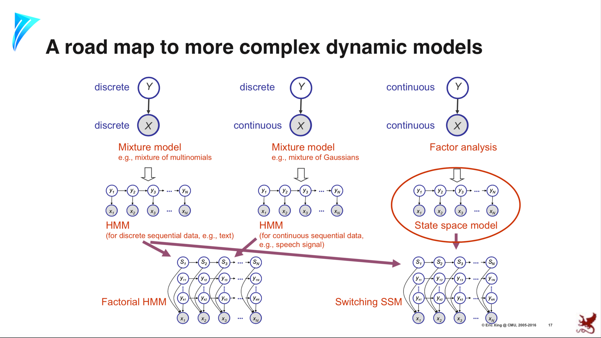
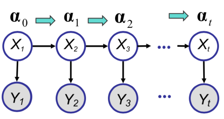
In the figure above, the dynamical (sequential) continuous counterpart to HMMs are the State Space Models (SSM). In fact, they are the sequential extensions of Factor Analysis discussed so far. SSM can be thought of as a sequential Factor Analysis or continuous state HMM.

Mathematically, let $f(\cdot)$ be any arbitrary dynamic model, and let $g(\cdot)$ be any arbitrary observation model. Then, we obtain the following equations for the dynamic system:

\begin{aligned} &x_t = f(x_{t-1}) + G w_t \\ &y_t = g(x_{t-1}) + v_t \end{aligned}

Here $w_t \sim \mathcal{N}(0, Q)$ and $v_t \sim \mathcal{N}(0, R)$ are zero-mean Gaussian noise. Further, if we assume that $f(\cdot)$ and $g(\cdot)$ are linear (matrices), then we get equations for a linear dynamical system (LDS):

\begin{aligned} &x_t = Ax_{t-1} + G w_t \\ &y_t = Cx_{t-1} + v_t \end{aligned}

An example of an LDS for 2D object tracking would involve observations $y_t$ to be 2D positions of the object in space and $x_t$ to be 4-dimensional, with the first two dimensions corresponding to the position and the next two dimensions corresponding to the velocity, i.e., the first derivative of the positions. Assuming a constant velocity model, we obtain the state space equations for this model, as shown below:

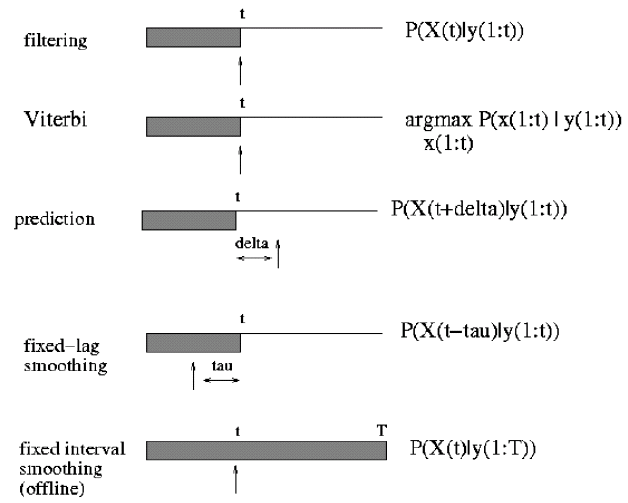
\begin{aligned} &\begin{bmatrix} x^1_t \\ x^2_t \\ \dot{x}^1_t \\ \dot{x}^2_t \end{bmatrix} = \begin{bmatrix} 1 & 0 & \Delta & 0 \\ 0 & 1 & 0 & \Delta \\ 0 & 0 & 1 & 0 \\ 0 & 0 & 0 & 1 \end{bmatrix} \begin{bmatrix} x^1_{t-1} \\ x^2_{t-1} \\ \dot{x}^1_{t-1} \\ \dot{x}^2_{t-1} \end{bmatrix} + \text{noise}\\ &\begin{bmatrix} y^1_t \\ y^2_t \end{bmatrix} = \begin{bmatrix} 1 & 0 & 0 & 0 \\ 0 & 1 & 0 & 0 \end{bmatrix} \begin{bmatrix} x^1_{t-1} \\ x^2_{t-1} \\ \dot{x}^1_{t-1} \\ \dot{x}^2_{t-1} \end{bmatrix} + \text{noise} \end{aligned}

There are two different inference problems that can be considered for SSMs:

The first problem is to infer the current hidden state ($x_t$) given the observations up to the current time $t$, i.e., $y_1, y_2, ..., y_t$. This problem is analogous to the forward algorithm in HMMs, is exact online inference problem, known as the $\textbf{Filtering}$ problem and will be discussed next.

Filtering
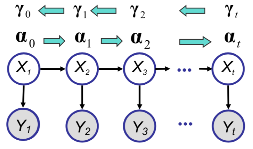
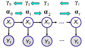
The second problem is the offline inference problem, i.e., given the entire sequence $y_1, y_2, ..., y_T$, estimate $x_t$ for $t < T$. This problem, called the $\textbf{Smoothing}$ problem, can be solved using the Rauch-Tung-Strievel algorithm and is the Gaussian analog of the forward-backward (alpha-gamma) algorithm in HMMs.

Smoothing

Kalman Filter

The Kalman Filter is an algorithm analogous to the forward algorithm for HMM. For the state space model (SSM), the goal of Kalman filter is to estimate the belief state $P(X_{t}|y_{1:t})$ given the data ${y_{1},…,y_{t}}$. To do so, it mainly follows a recursive procedure that includes two steps, namely time update and measurement update. Here, we are going to derive the two steps.

Derivation

Time Update:

(1) Goal: Compute $P(X_{t+1}|y_{1:t})$ (the distribution for $X_{t+1|t}$) using prior belief $P(X_{t}|y_{1:t})$ and the dynamical model $P(X_{t+1}|X_{t})$.

(2) Derivation: Recall that the dynamical model states that $X_{t+1}=AX_{t}+Gw_{t}$ where $w_{t}$ is the noise term with a Gaussian distribution $\mathcal{N}(0; Q)$. Then, we can conpute the mean and variance for $X_{t+1}$ using this formula.

For the mean, we have:

\begin{aligned} \hat{X}_{t+1|t} & = \mathbb{E}(X_{t+1}|y_{1},...,y_{t})\\ & = \mathbb{E}(AX_{t}+Gw_{t})\\ & = A \hat{X}_{t|t} \end{aligned}

For the variance, we have:

\begin{aligned} P_{t+1|t} & = \mathbb{E}((X_{t+1}-\hat{X}_{t+1|t})(X_{t+1}-\hat{X}_{t+1|t})^T|y_{1},...,y_{t})\\ & = \mathbb{E}((AX_{t}+Gw_{t}-\hat{X}_{t+1|t})(AX_{t}+Gw_{t}-\hat{X}_{t+1|t})^T|y_{1},...,y_{t})\\ & = AP_{t|t}A^T+GQG^T \end{aligned}

Measurement Update:

(1) Goal: Compute $P(X_{t+1}|y_{1:t+1})$ using $P(X_{t+1}|y_{1:t})$ computed from time update, observation $y_{t+1}$ and observation model $P(y_{t+1}|X_{t+1})$.

(2) Derivation: The key here is to first compute the joint distribution $P(X_{t+1},y_{t+1}|y_{1:t})$, then derive the conditional distribution $P(X_{t+1}|y_{1:t+1})$. Recall that the observation model states that $y_{t}=CX_{t}+v_{t}$ where $v_{t}$ is the noise term with a Gaussian distribution $\mathcal{N}(0; R)$. We have already computed the mean and the variance of $X_{t+1|t}$ in the time update. Now we need to compute the mean and the variance of $y_{t+1|t}$ and the covariance of $X_{t+1|t}$ and $y_{t+1|t}$.

For the mean of $y_{t+1|t}$, we have:

\begin{aligned} \hat{y}_{t+1|t} & = \mathbb{E}(y_{t+1}|y_{1},...,y_{t})\\ & = \mathbb{E}(CX_{t+1}+v_{t+1})\\ & = C \hat{X}_{t+1|t} \end{aligned}

For the varaince of $y_{t+1|t}$, we have:

\begin{aligned} \mathbb{E}((y_{t+1}-\hat{y}_{t+1|t})(y_{t+1}-\hat{y}_{t+1|t})^T|y_{1},...,y_{t}) & = \mathbb{E}((y_{t+1}-C \hat{X}_{t+1|t})(y_{t+1}-C \hat{X}_{t+1|t})^T|y_{1},...,y_{t})\\ & = C P_{t+1|t} C^T + R \end{aligned}

For the covaraince of $X_{t+1|t}$ and $y_{t+1|t}$, we have:

\begin{aligned} \mathbb{E}((y_{t+1}-\hat{y}_{t+1|t})(X_{t+1}-\hat{X}_{t+1|t})^T|y_{1},...,y_{t}) = C P_{t+1|t} \end{aligned}

Hence the joint distribution of $X_{t+1|t}$ and $y_{t+1|t}$ is:

\mathcal{N}(\begin{bmatrix} X_{t+1|t} \\ y_{t+1|t} \end{bmatrix} | \begin{bmatrix} \hat{X}_{t+1|t} \\ C\hat{X}_{t+1|t} \end{bmatrix}, \begin{bmatrix} P_{t+1|t} & P_{t+1|t}C^T \\ CP_{t+1|t} & C P_{t+1|t} C^T + R \end{bmatrix})

Finally, to compute the conditional distribution of a joint Gaussian distribution, we recall the formulas as:

\begin{aligned} m_{1|2} & = \mu_1+\Sigma_{12}\Sigma_{22}^{-1}(x_2-\mu_2) \\ V_{1|2} & = \Sigma_{11}-\Sigma_{12}\Sigma_{22}^{-1}\Sigma_{21} \end{aligned}

Plugging in results from above we have the conditional distribution of $P(X_{t+1}|y_{1:t+1})$ as:

\begin{aligned} \hat{X}_{t+1|t+1} & = \hat{X}_{t+1|t} + K_{t+1}(y_{t+1}-C\hat{X}_{t+1|t}) \\ P_{t+1|t+1} & = P_{t+1|t} - K_{t+1} C P_{t+1|t} \end{aligned}

where $K_{t+1} = P_{t+1|t}C^T(CP_{t+1|t}C^T+R)^{-1}$ is referred to as the Kalman gain matrix.

Example

We now see an example of Kalman filter on a problem on noisy observations of a 1D particle doing a random walk. The SSM is given as:

\begin{aligned} X_{t+1|t} & = X_{t} + w \\ y_{t} & = X_{t} + v \end{aligned}

where $w \sim \mathcal{N}(0; \sigma_{x})$ and $v \sim \mathcal{N}(0; \sigma_{y})$ are noises. In other words, $A=G=C=I$. Thus, using the update rules derived above we have that at time t:

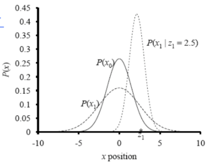
\begin{aligned} P_{t+1|t} & = \sigma_{t}+\sigma_{x} \\ \hat{X}_{t+1|t} & = X_{t|t} \\ K_{t+1} & = (\sigma_t+\sigma_x)(\sigma_t+\sigma_x+\sigma_y)\\ \hat{X}_{t+1|t+1} & = ((\sigma_t+\sigma_x)y_t+\sigma_y\hat{X}_{t|t})/(\sigma_t+\sigma_x+\sigma_y)\\ P_{t+1|t+1} & = ((\sigma_t+\sigma_x)\sigma_y)/(\sigma_t+\sigma_x+\sigma_y) \end{aligned}

As demonstrated in the figure below, given prior belief $P(X_0)$, our estimate of $P(X_1)$ without an observation has the same mean and larger variance as shown by the first two lines in equations above. However, given an observation of $2.5$, the new estimated distribution shifted to the right accoding to last three lines of equations above.

1D Kalman Filter example

Complexity of one KF step:

Let $X_t \in R^{N_x}$ and $Y_t \in R^{N_y}$

Predict step: $P_{t+1|t} = AP_{t|t}A + GQG^T$

This invloves matrix multiplication of $N_x$ x $N_x$ matrix with another $N_x$ x $N_x$ matrix, hence the time complexity is $O(N_{x}^{2})$

Measurement Updates: $K_{t+1} = P_{t+1|t}C^T(CP_{t+1|t}C^T + R)^{-1}$

This invloves a matrix inversion of $N_y$ x $N_y$, hence the time complexity is $O(N_{y}^{3})$

Overall time = max{$N_{x}^{2},N_{y}^{3}$}

Rauch-Tung-Strievel

The Rauch-Tung-Strievel algorithm is a Gaussian analog of the forwards-backwards(alpha-gamma) algorithm for HMM. The intent is to estimate $P(X_t|y_{1:T})$.

Rauch-Tung-Strievel

Since, $P(X_t|y_{1:T})$ is a Gaussian distribution, we intend to derive mean $X_{t|T}$ and variance $P_{t|T}$.

Let’s first define the joint distribution $P(X_{t},X_{t+1}|y_{1:t})$.

m = \begin{bmatrix} \hat{x}_{t|t} \\ \hat{x}_{t+1|t} \end{bmatrix}, V = \begin{bmatrix} P_{t|t} & P_{t|t}A^T \\ AP_{t|t} & P_{t+1|t} \end{bmatrix}

where m and V are mean and covariance of joint distribution respectively.

We are going to use a neat trick to arrive at the RTS inference.

$E[X|Z] = E[E[X|Y,Z]|Z]$

$Var[X|Z] = Var[E[X|Y,Z]|Z] + E[Var[X|Y,Z]|Z]$

Now, applying these results to our problem:

\hat{x}_{t|T} = E[X_t|Y_{1:T}] = E[E[X_t|X_{t+1},Y_{1:T}]| Y_{1:T}]

$X_t$ is independent of $X_{t+2:T}$ given $X_{t+1}$, so:

\begin{aligned} \hat{x}_{t|T} & = E[E[X_t|X_{t+1},Y_{1:t}]| Y_{1:T}] \\ & = E[X_t|X_{t+1},Y_{1:t}] \end{aligned}

Using the formulas for the conditional Gaussian distribution:

\hat{x}_{t|T} = \hat{x}_{t|t} + L_t(\hat{x}_{t+1|T} - \hat{x}_{t+1|t})

Similarly,

P_{t|T} = Var[\hat{X}_{t|T} | y_{1:T}] + E[Var[X_t|X_{t+1},y_{1:t}]|y_{1:T}]

where, $L_t = P_{t|t}A^TP^{-1}_{t+1|t}$

Learning State Space Model

Likelihood:

\begin{aligned} \mathcal{l}(\theta,D) & = \sum_n log(p(x_n,y_n)) = \sum_n log(p(x_1) + \sum_n \sum_t log(p(x_{n,t}|x_{n,t-1})) + \sum_n \sum_t log(p(y_{n,t}|x_{n,t})) \\ & = f_1(X_1,\sum_0) + f_2(\{X_tX_{t-1}^T, X_tX_t^T,X_t:\forall t \};A,Q,G) + f_3(\{X_tX_t^T,X_t : \forall t\};C,R) \end{aligned}

E-step: Compute $<X_tX_{t-1}^T>$, $<X_tX_t^T>$ and $<X_t>$ using Kalman Filter and Rauch-Tung-Strievel methods.

M-step: Same as explained in the Factor Analysis section.

Non-Linear Systems

In some of the real world scenarios, the relation between model states as well as states and observations may be non-linear. This renders a closed form solution to the problem almost impossible. In recent works, this non-linearity relation is captured using deep neural networks and stochastic gradient descent based methods are used to obtained the solutions. These state space models can be represented as:

$x_t = f(x_{t-1}) + w_t$

$y_t = g(x_t) + v_t$

Since the effect of the noise covariance matrices Q and R remains unchanged due to non-linearity, they have been omitted from the discussion for convenience.

An approximate solution without using deep neural networks is to express the non-linear functions using Taylor expansion. The order of expansion depends on the use case and the extent of the non-linearity. These are referred to as Extended Kalman Filters. The following equations show the second order Taylor expansion for Extended Kalman Filters:

x_t = f(\hat{x}_{t-1|t-1}) + A_{\hat{x}_{t-1|t-1}}(x_{t-1} - \hat{x}_{t-1|t-1}) + w_t

y_t = g(\hat{x}_{t|t-1}) + C_{\hat{x}_{t|t-1}}(x_{t} - \hat{x}_{t|t-1}) + v_t

where,

\hat{x}_{t|t-1} = f(\hat{x}_{t-1|t-1})

A_{\hat{x}} = \frac{\partial f}{\partial x}

C_{\hat{x}} = \frac{\partial g}{\partial x}

Online vs Offline Inference

Online Inference: Inference methods that are based on looking only at the observations till the current time-step. They generally take the form $P(X|y_{1:t})$. The inference objective may vary depending on the algorithm. Eg, Kalman Filter.

Offline Inference. Inference methods than consider all the observations from all the time-steps. The take the form $P(X|y_{1:T})$. Eg, Rauch-Tung-Strievel smoothing.

Online vs Offline Learning

Recursive Least Squares and Least Mean Squares

Consider a special case where the state $x_t$ remains constant while the observation coefficients ($C$) vary with time. In this scenario, observations are affected by the coefficients rather than the state itself. This turns the estimation of the state into a linear regression problem.

Let $x_t = \theta$ and $C = x_t$ in the KF update equation. Then we can represent the observation models as

$y_t = x_t\theta + v_t$

which takes exactly the form of a linear regression problem to estimate $\theta$.

Now, using the Kalman Filter idea we can formulate the update equation for this problem as:

\hat{\theta}_{t+1} = \hat{\theta_{t}} + P_{t+1}R^{-1}(y_{t+1}-x^T\hat{\theta_t})x_t

This is the recursive least squares algorithm as one can see that the update term takes the form of the derivative of square of the difference. If we treat $\eta = P_{t+1}R^{-1}$ as a constant this exactly becomes least mean squares algorithm.

\hat{\theta}_{t+1} = \hat{\theta_{t}} + \eta(y_{t+1}-x_t^T\hat{\theta_t})x_t