Lecture 11: Kalman Filtering and Topic Models
Kalman Filtering and Topic Models. See abstract. Due to the previous lecture running over, the actual material covered in the lecture deviated from what the lecture schedule suggests.
Note on Lecture Content
Due to the previous lecture running over, the actual material covered in the lecture deviated from what the title of the lecture on the course homepage suggests.
Introduction
In the previous lecture, we introduced State Space Models which can be visualized as sequential FA (Factor Analysis) models or HMMs (Hidden Markov Models) where both hidden states and outputs are drawn from continuous distributions. State space models are linear dynamic systems. However, due to time constraints, we were unable to discuss techniques to perform efficient inference on these models.
In this lecture, we pick up from the previous lecture and first cover Kalman Filtering, a recursive algorithm for inference in State space models and derive equations for this technique. We then look at an example of Kalman Filtering on a toy 1-D problem and gain a deeper understanding of the intuition behind it. Finally, we take a brief look at how to perform parameter learning for state space models and how to deal with non-linearity in these systems. After this, we move on to the topic of approximate inference (the originally intended topic for today’s lecture). So far, all inference techniques we have seen through the course have been exact inference techniques. However, in this portion of the lecture, we discuss a setting where exact inference is unfeasible: Topic Models. We describe the motivation behind building topic models and develop a mathematical representation for these models. From our representation, we see that performing exact inference on these models is super-exponential and so we introduce two approximate inference techniques to handle this: Variational Inference and Markov Chain Monte Carlo. This lecture only covers variational inference and the mean-field assumption in topic models.
Kalman Filtering
Kalman filtering is a technique to perform efficient inference in the forward algorithm for state-space models. Consider the following state-space model:
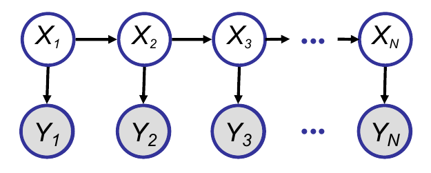
As we can see, this model consists of a sequence of hidden states, with each hidden state emitting an observation. To perform inference efficiently on this model, we can define a recursive algorithm as follows:
- Compute $ P(X_t \vert Y_{1…t}) $
- Compute $ P(X_t+1 \vert Y_{1…t+1}) $ from the previous probability after adding the observation $ Y_{t+1} $
Kalman filtering provides a way of performing this recursion. It breaks the computation into two steps:
- Predict Step: Compute $P(X_{t+1} \vert Y_{1…t})$ (prediction) from $ P(X_t \vert Y_{1…t}) $ (prior belief) and $P(X_{t+1} \vert X_t)$ (dynamical model)
- Update Step: Compute $P(X_{t+1} \vert Y_{1…t+1})$ from $P(X_{t+1} \vert Y_{1…t})$ (prediction), $Y_{t+1}$ (observation) and $P(Y_{t+1} \vert X_{t+1})$ (observation model)
The predict and update steps are also called the time update and measurement update steps respectively. We will now derive equations for both steps for our state-space model. Remember that all hidden states and observations in the model are drawn from Gaussian distributions since they are computed via linear transformations. This means that all conditional and marginal probabilities in the model are also Gaussian distributions.
Predict Step Derivation
Remember that the dynamical model is defined as $X_{t+1} = AX_t + GW_t$, where $W_t \sim \mathcal{N}(0,Q)$ We can compute the mean and variance for this Gaussian distribution as follows:
For the observation model, which is defined as $Y_{t} = CX_t + \nu_t$, where $\nu \sim \mathcal{N}(0,R)$, we can compute the mean and variance as follows:
Finally, we can also derive the following:
\[E((Y_{t+1} - \hat Y_{t+1 \vert t})(X_{t+1} - \hat X_{t+1 \vert t})^T \vert Y_1...Y_t) = CP_{t+1|t}\]Update Step Derivation
Recall that for two gaussian distributions $X_1, X_2$, their joint distribution is a Gaussian with the following mean and variance:
Using this result in combination with the derivations from the predict step, we can deduce that $P(X_{t+1}, Y_{t+1} \vert Y_1…Y_t) \sim \mathcal{N}(M_{t+1}, V_{t+1})$, where
Given a joint distribution of two Gaussian random variables $X_1, X_2$, recall that their conditional and marginal probability distributions are defined as follows:
Using this information, we can compute the measurement update (update step) as:
Here $K_{t+1} = P_{t+1 \vert t} C^T (C P_{t+1 \vert t} C^T + R)^{-1}$ and is known as the Kalman gain matrix. An interesting point to note is that $K_t$ is independent of $Y_t$ (i.e. the data), so it can be precomputed to improve efficiency.
Example of Kalman Filtering in 1-D
Suppose we have some noisy observations of a particle performing a random walk in 1-D. Assume our states and observations are defined as follows:
$ X_{t \vert t-1} = X_{t-1} + W $ where $W \sim \mathcal{N}(0,\sigma_x)$
$ Z_{t} = X_{t} + V $ where $V \sim \mathcal{N}(0,\sigma_z)$
We can compute KF updates for this model as follows:
Understanding the intuition behind Kalman Filtering
In the KF update equation for the mean, $\hat X_{t+1 \vert t+1} &= \hat X_{t+1 \vert t} + K_{t+1} (Z_{t+1} - C \hat X_{t+1 \vert t})$, the term $(Z_{t+1} - C \hat X_{t+1 \vert t})$ is called the innovation term. We can see that the update equation for new belief is a convex weighted combination of updates from prior and observation, with the Kalman Gain matrix acting as the weight. From the equation for the Kalman Gain matrix, we can see that if observations are noisy ($\sigma_z$ or $R$ is large), then the KG matrix is small and updates rely more on prior. On the other hand if the process is unpredictable (large $\sigma_x$) or prior is unreliable (large $\sigma_t$), the KG matrix is higher and we rely more on the observation.
High-level Discussion of the Derivation of the A, G, and C Matrices
Note: content from this section is from a two-minute digression from Dr. Xing responding to a student’s question. As such, it is not in depth but only meant to add context. For more details about learning in this situation, see the sections that follow, and previous lectures on EM.
Up to this point, we have discussed inference in the Kalmann filter model; given the model up-front, tell me something about the data. This leaves open where the matrices A, G, and C come from, however. This is a similar situation we were in for HMMs: to find the necessary matrices, we must do learning. Using approaches like EM we can interleave learning and inference to come across the parameters of interest.
Furthering this comparison to HMMs, the Rauch-Tung-Strievel algorithm allows us to perform “exact off-line inference in an LDS”, and is essentially a “Guassian analog of the forwards-backwards” algorithm. While it is good to know of the existance of this latter algorithm, we will not cover it in detail in this course, since the principles are very similar to before, and appropraite resources exist for those interested in learning more.
Learning State Space Models (SSMs)
In order to learn the necessary parameters for the Kalmann filter, we calculate the complete data likelihood:
This is very similar to what we saw in factor analysis, except there, we computed this for each individual time-step, whereas here we do it for all time-steps. From here, we proceed as usual in EM: in the E-step, we estimate $X_tX_{t-1}^{T}$, $X_tX_t^{T}$, and $X_t$ by taking their expectation in respect to the observation, and in the M-step we use MLE in the typical fashion.
Non-Linear Systems
The approaches discussed thus far are designed to handle linear systems. In order to handle a non-linear system, an approximation must be made. For example, for non-linear differentiable systems, Taylor expansion allows us to use linear terms to approximate non-linear curves.
With that, we close the modeling section of the course and move on to the next subject.
Approximate Inference and Topic Models: Mean Field and Loopy Belief Prop
Thus far in the course, we have covered the elimination algorithm, message passing, and algorithms that are powered based on those principles. These techniques allowed for exact inference, and while they have been shown useful, they cannot cope with many of the settings and problems we wish to explore. This motivates uses of approximate techniques, which we will begin discussing in this lecture.
Appropriately Modeling Different Tasks
With contemporary excitement about ML and particularly Deep Models, it is not uncommon for students to want to select a model that interests them and try to apply it to some difficult tasks. It is typically more appropriate and sound to go the other way - find the right model and methods to handle a task at hand.
To begin discussion of the next subject and motive its development, we consider the problem of trying to given someone a summary, a “bird’s-eye view”, or one million or more documents. That is our task - we know at some point, to get a handle on it, we have to convert it to mathematical language. To do this, we have to consider a framework to put it in mathematically. Is this a classification task? No, we have not even discussed labels. Is it a clustering task? Maybe, but the cluster-label itself would be very weakly informative of what is actually going on in the documents. Embeddings, representing each document as a point in a space or plane? Maybe. One has to decide on this matter to move forward.
Another point to decide is representation of the data. We want to deal with text ultimately, which is a sequence of words. How do we want to represent that? Binary vectors? Counts? This is a design choice one must consider.
After deciding the task and the data representation, one may consider a model to fit these. From there, one can consider how inference can be done on the model. After that, how learning can be accomplished may be considered so that parameters to the model may be filled in an informed fashion. Finally, after all the modeling and processing is done, results may be evaluated to get a sense of how well our methods are doing. In general, it is best to handle each step of this process one at a time. This is part of the art of modeling.
Motivating Example: Probabilistic Topic Model
Probabilistic topic model is used here to demonstrate the challenge with inference on graphic models and the necessity of approximate inference.
Problem Motivation:
It is difficult for human to handle a large number of textual documents. It would be helpful to automate some of such processes, such as search, browse or measure similarity.
A specific task is document embedding, i.e. finding low-dimensional representation of documents. Furthermore, it is desirable that the latent representation corresponds to semantic meaning, such as topics. One approach to such a representation is to look at frequent words that corresponds to a topic.
Using the embedding, one application is to study the evolution of documents over time. Another application is to track user interest based on his/her posts on social media.
Representation:
Bag of words representation is the starting point of topic modeling. Specifically, each document is represented as a vector in word space, i.e. count of each word in the dictionary.
The main advantage of this method is simplicity. The limitation is that the ordering of words is neglected. To give an example: two documents of different length is not comparable under a representation based on word ordering. The longer document has smaller likelihood by taking the product of a longer sequence. Under the bag of words representation, any two documents would be vectors of same length and thus comparable.
Documents are usually represented as very long vectors under bag of words, due to the large size of the dictionary. The representation can be more compact with topic modeling.
To model semantic meaning in a document, one look at keywords that correspond to a specific topic. Figure 1 provides a concrete example. Keywords such as “source”, “target” and “BLEU” show that the document is about machine translation. The document also contains vocabulary associated with topic such as syntax and learning.
Furthermore, one can assign probability to each topic. In this example, keywords on machine translation are most frequent, so we assign a larger probability. There is some mention related to syntax and learning, so we assign some probability based on word frequency.
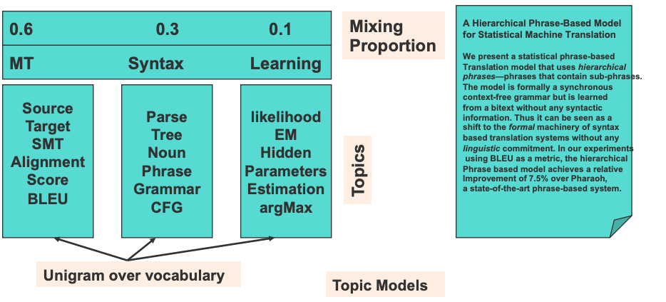
To sum up, a document is first represented with bag of words. Then, the bag of words representation is transformed into strength on topics, which is a very compact representation.
Topic Models:
The probability of each word in a document, $P(w)$, can be decomposed into the distribution of topics in a document, $P(z)$, and the probability of a word given the topic, $P(w|z)$.
\[P(w) = P(w|z)P(z)\]A related concept is latent semantic indexing (LSI). LSI decomposes matrix with linear algebra-based method. However, the drawback of LSI, which involves matrix inversion, is high computational cost.
The architecture of topic model is shown in Figure 2. To sample from a document, one first draw a topic distribution $\theta$ based on the prior. For a document with $N_d$ words, one first draw topic indicators, z, from topic distribution, $\theta$. Then one draws words, w, from word-frequency distribution, K, conditioning on the topic indicator, z.
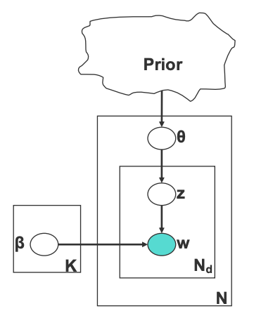
Having decided on the architecture, we need to make more specific modeling choices, i.e. the distributions to sample from. In typical implementation, we draw z from a multinomial distribution, parameterized by $\theta$. The word distribution conditioned on topic is also drawn from a multinomial distribution, parameterized by $\beta$. The most commonly used prior is Dirichlet, because it is a conjugate prior of multinomial distribution. One limitation of Dirichlet is that it does not allow for modeling the relationship between different topics. An alternate approach is to use a logistic-normal as prior.
Doing Inference on Topic Models
To perform inference on our topic models, we start by considering the joint likelihood based on the hidden and observed random variables. Leveraging the graph structure we have for topic models, we can factorize this distribution in the fashion we are used to.
\[p(\beta, \theta, z, w) = \Pi_{k=1}^{K}p(\beta_k | \eta)\Pi_{d = 1}^{D}p(\theta_d | \alpha) \Pi_{n = 1}^{N}p(z_{d_n}|\theta_d)p(w_{d_n} | z_{d_n}, \beta)\]Given a query, answering the above joint would require marginalizing out the variables and values that do not interest us - but doing so would require super-exponential work in this model, integrating across variables that may have a large set of possible values. Thus, our typical approach is not tractable here.
This motivates approximate inference: we trade off exact computation for reasonable computational work. We will cover two major families of methods in this lecture and next: Variational Inference and Markov Chain Monte Carlo.
Variational Inference
Variational inference is a technique that allows one to convert an inference problem into an optimization problem. We want to maximize the data likelihood, but as we already discussed, that itself is too hard to handle. Thus, we begin by lower-bounding the data likelihood with a term known as the “free-energy”.
We start by introducing another distribution , $Q_{\phi}$ which is a distribution on the same set of random variables. The goal, eventually, is to have $Q_{\phi}$ be a distribution that is easier to work with than $p$ but is sufficiently “close” to serve as a reasonable surrogate in calculations.
Using this, we want to maximize the lower bound for the log-likelihood:
Equivalently, we can minimize the aforementioned “free-energy” of the system:
\[F(\theta, \phi ; x) = -\log(p(x)) + KL(Q_{\phi}(z | x) || p_{\theta}(z | x))\]Intuitively, the connection between $\mathscr{L}(\theta, \phi ; x)$ and $F(\theta, \phi ; x)$ is that the $KL$ divergence measures the gap between the lower bound on the likelihood ($\mathscr{L}$) and the real likelihood ($\log(p(x))$) - both the minimization and the maximization noted above try to close that gap.
We call $\mathscr{L}(\theta, \phi ; x)$ above the variational lower bound. Often it is written as
\[\mathscr{L}(\theta, \phi ; x) = \log(p(x)) - KL(Q_{\phi}(z | x) || p_{\theta}(z | x)),\]which simply is $\mathscr{L}(\theta, \phi ; x) = -F(\theta, \phi ; x)$.
Mean-Field Assumption (In Topic Models)
Recall the form of the true posterior:
\[p(\beta, \theta, z | w) = \frac{p(\beta, \theta, z, w)}{p(w)}\]Suppose that in $Q$ (our approximation to $p$) we could break dependancies in the joint by assuming a so-called “fully-factorized” distribution is followed, i.e.:
\[Q(\beta, \theta, z) = \Pi_{k}Q(\beta_k)\Pi_{d}Q(\theta_d)\Pi_{n}Q(z_{d_n})\]Notice that in this fully-factored model, each factor is a term of an unconditional distribution - this is unlike the factorization we say over Bayes Nets before, where conditional distributions appear, complicating the marginalization process. As such, if we need to answer a query of form $Q(z_d)$, marginalizing across $Q(\beta, \theta, z)$ is trivial since we now that moving the sums into the product, $\sum_{\theta, \beta}\Pi_{k}Q(\beta_k)\Pi_{d}Q(\theta_d) = 1$, allowing us to answer the query using only the marginals for $z_d$ under $Q$ that we suppose we already have on hand. That is, marginalizing variables out under distribution $Q$ no longer becomes necessary in many or all cases- we know a priori that the joint over any subset of the variables under such a $Q$ will simply be the produce of those variables’ marginals.
In general with variational methods, the true posterior for our target distribution, $p$,
might not exist in the family of $Q$ we consider - we buy tractability at the cost
of irreducible approximation error.
For further reference, take a look at the original LDA paper