Lecture 12: Theory of Variational Inference: Marginal Polytope, Inner and Outer Approximation
Introduction of Loopy Belief Propagation algorithm and the theory behind it and Mean-field approximation.
Recap of the message passing algorithm and its properties
In the previous lectures, we have looked at exact inference algorithms and observed that they are not very efficient. Hence, a need for more efficient inference algorithms arises. This lecture will focus on such algorithms which are called Approximate Inference Algorithms.
Inference using graphical models can be used to compute marginal distributions, conditional distributions, the likelihood of observed data, and the modes of the density function. We have already studied that exact inference can be accomplished either using brute force (i.e. eliminating all the required variables in any order) or by refining our elimination order so as to reduce the number of computations. In this context, the belief propagation or sum-product message passing algorithm run on a clique tree generated by a given variable elimination ordering was introduced as an equivalent way of performing variable elimination. We have seen that the overall complexity of the algorithm is exponential in the number of variables in the largest elimination clique which is generated when we use a given elimination order. The tree width of a graph was defined as one less than the smallest possible value of the cardinality of the largest elimination clique, ranging over all possible elimination orderings. If we can find an optimal elimination order, we can reduce the complexity of belief propagation. As the problem of finding the best elimination order is NP-hard, exact inference is also NP-hard. Belief propagation is guaranteed to converge to a unique and fixed set of values after a finite number of iterations when it is run on trees.
For more details about the message passing algorithm, please look at the Notes for Lecture 4.
Message Passing Protocol
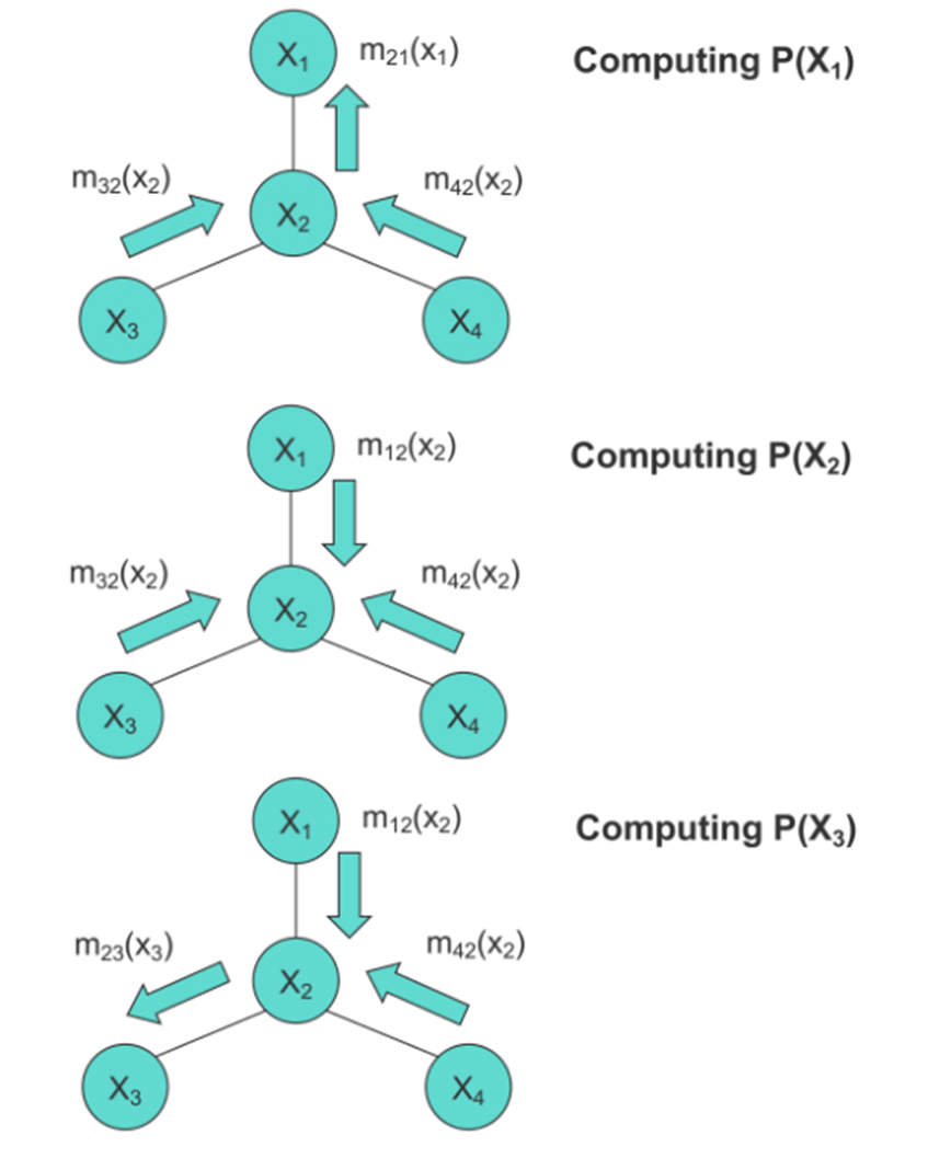
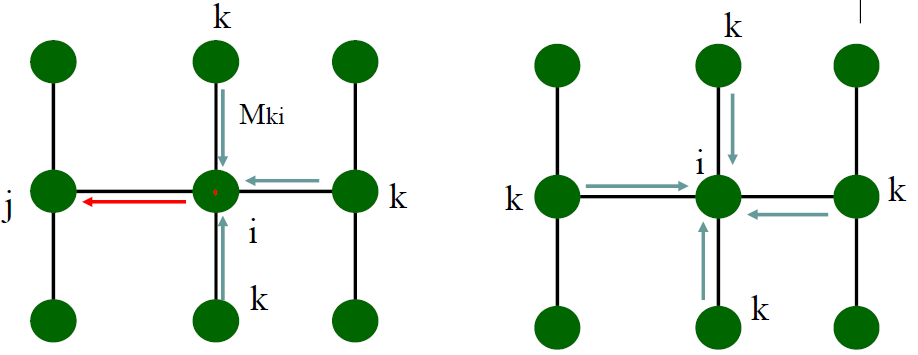
The message passing protocol dictates that a node can only send a message to its neighbors when and only when it has received the messages from all of its other neighbors. Hence, to naively compute the marginal of a given node, we should treat that node as the root and run the message passing algorithm. This is illustrated by the three figures given below, each of which shows the messaging directions to be used when computing the given marginal:
Message Passing for HMMs
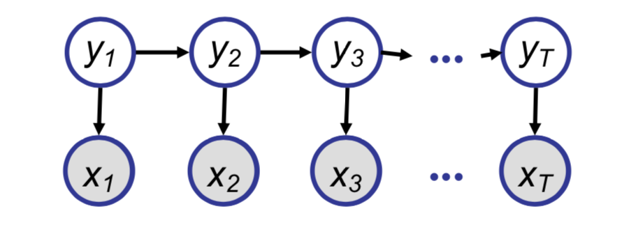
When the message passing algorithm is applied to a HMM shown below, we will see that the forward and backward algorithms can be obtained.
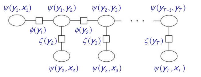
The corresponding clique tree for the HMM shown above is:
Now, the messages (denoted by \(\mu\)s) and the potentials (denoted by \(\psi\)s) involved in the rightward pass are depicted by the below figure:
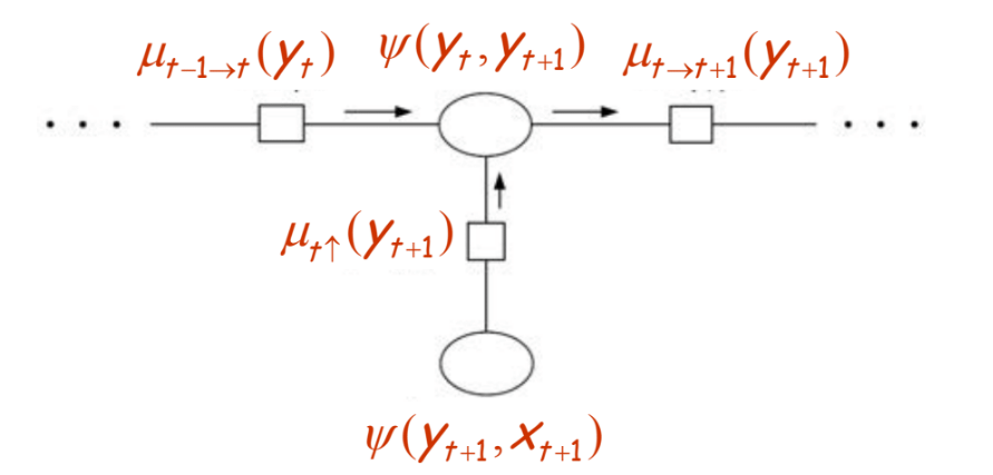
We have that,
\[\mu_{t\rightarrow t+1} (y_{t+1}) = \sum_{y_t} \psi(y_t,y_{t+1})\mu_{t-1\rightarrow t}(y_t)\mu_{t\uparrow}(y_{t+1})\]We know that:
\[\psi(y_t,y_{t+1}) = p(y_{t+1}|y_t) = a_{y_t,y_{t+1}}\]is the probability of transitioning from \(y_t\) to \(y_{t+1}\) and
\[\mu_{t\uparrow}(y_{t+1}) = p(x_{t+1}|y_{t+1})\]is the probability of emitting \(x_{t+1}\) in state \(y_{t+1}\).
\[\Longrightarrow \mu_{t\rightarrow t+1} (y_{t+1}) = \sum_{y_t} p(y_{t+1}|y_t)\mu_{t-1\rightarrow t}(y_t)p(x_{t+1}|y_{t+1}) = p(x_{t+1}|y_{t+1}) \sum_{y_t} a_{y_t,y_{t+1}} \mu_{t-1\rightarrow t}(y_t)\]which is the forward algorithm.
Similarly, the messages and the potentials involved in the leftward pass are depicted by the below figure:
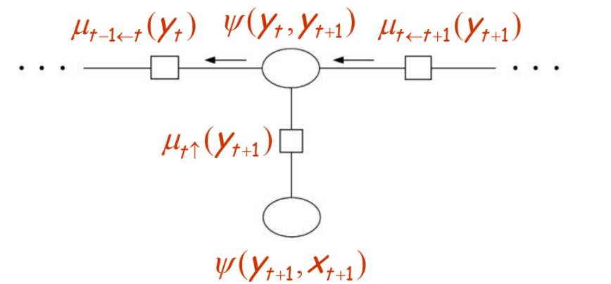
Then we have that,
\[\mu_{t-1\leftarrow t}(y_t) = \sum_{y_{t+1}} \psi(y_t,y_{t+1}) \mu_{t\leftarrow t+1}(y_{t+1})\mu_{t\uparrow}(y_{t+1}) = \sum_{y_{t+1}} p(y_{t+1}|y_t) \mu_{t\leftarrow t+1}(y_{t+1}) p(x_{t+1}|y_{t+1})\]which is the backward algorithm.
Correctness of Belief Propagation in Trees
Theorem: The message passing algorithm correctly computes all of the marginals in a tree.
This is a result of there being only one unique path between any two nodes in a tree. Intuitively, this guarantees that only two unique messages can be associated with an edge, one for each direction of traversal.
Local and Global Consistency
Let \(\{\tau_C, C \in \mathcal{C}\}\) and \(\{\tau_S, S \in \mathcal{S}\}\) denote the set of functions which are associated with cliques and separator sets respectively.
These sets of functions are locally consistent if the following properties hold:
- \[\sum_{x'_S} \tau_S(x'_S) = 1, \forall S \in \mathcal{S}\]
- \[\sum_{x'_C|x'_S = x_S} \tau_C(x'_C) = \tau_S(x_S), \forall C \in \mathcal{C}, \forall S \subset C\]
The first property implies that the functions associated with each separator set are proper marginals. The second property requires that if we sum any clique function \(\tau_C\) over all the variables in the clique \(C\) which are not present in a sepset \(S \subset C\), we must obtain a function \(\tau_S(X_S)\).
The aforementioned sets of functions are global consistent if all \(\tau_C\) and \(\tau_S\) are valid marginals.
For junction trees, local consistency is equivalent to global consistency. A proof of this fact can be found at this link.
However, for graphs which are not trees, local consistency does not always imply global consistency.
Example
Consider the two following message passing sequences for the same graph:
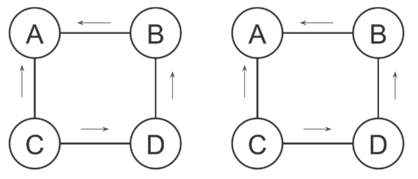
It can be seen that we obtain different values for \(P(A)\) based on the message passing sequence.
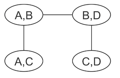
Similarly, if we construct a clique tree for the above graph (shown below), we see that the random variable \(C\) is part of two non-neighbouring cliques. Hence, it is impossible for the two clique potentials which contain \(C\) to agree on the marginal associated with \(C\) since no information about \(C\) is ever passed in the messages.
Loopy Belief Propagation
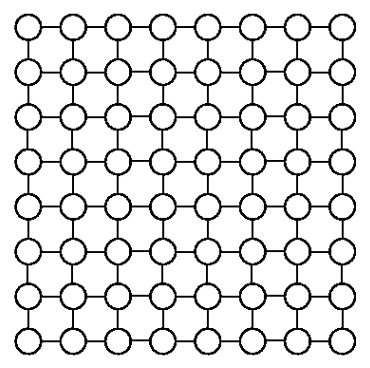
Above examples illustrate that on a non-tree graphical model the message passing algorithms are not guaranteed to provide a correct solution to the inference problem anymore. One way to deal with this is to convert a non-tree graphical model into a junction tree. However, such conversion often leads to graph with extremely large tree-width which is also unaffordable. For example in the following figure, an Ising model with \(N \times N\) grid and \(N\sim O(1000)\) will yield a clique with \(2^{100}\) entries. Therefore, we have to do approximation inference such as loopy belief propagation or mean field approximation.
Introduction to loopy Belief propagation and empirical observations
The main idea of loopy belief propagation does is to extend belief propagation algorithm (a.k.a message passing algorithm) from tree to non-tree graphical models. Considering an undirected graphical model with pairwise and singleton potential functions, the loopy belief propagation algorithm calculates the messages and marginal probability based on the following equations:
To be specific, the messages are updated and passed iteratively among nodes at the same time. Different from belief propagation algorithm where we pass the messages from the leaves to the root, the message passing here is recurrent. Another difference is that the loopy belief propagation algorithm doesn’t need to pass messages only after collecting all the messages from its neighbors. Previous studies showed that directly copying the idea of belief propagation from tree to non-tree graphical model leads to two outcomes:
- The algorithm converges and the approximated results are usually close to the results calculated by brute-force marginalization of variables.
- The algorithm fails to converge at all and oscillates between multiple answers of \(b\).
A theory behind loopy belief propagation: Bethe approximation to Gibbs free energy
It is often the case to use a distribution Q to approximate the intractable distribution P. In order to obtain a good approximation, the KL-divergence between Q and P is supposed to be reasonably small. Based on the factorized probability of the joint distribution, we can write the KL-divergence between Q and P as follows:
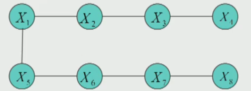
We call the first two terms \(-H_Q(X)-\sum_{f_\alpha\in F}E_Q\log f_\alpha(X_\alpha)\) the Free Energy. Now we consider an example of tree-structured distribution shown above. Based on the chain rule and local Markov property of undirected graphical model, we can expand the joint probability to factorized probability. According to the Bayes rule, we can further write the joint probability in the following form:
Note that only the singleton probabilities \(P(X_1)\) and \(P(X_8)\) don’t occur in the above equations. Therefore, we can summarize the joint probability for any tree-structured distribution as \(b(x)=\prod_{\alpha}b_{\alpha}(x_{\alpha})\prod_ib_i(x_i)^{(1-d_i)}\), where \(d_i\) represents the degree of that note \(x_i\). With this probability and the definition of the Free Energy, we can further write the entropy term and Free Energy as follows:
Then we consider a non-tree graph like this:
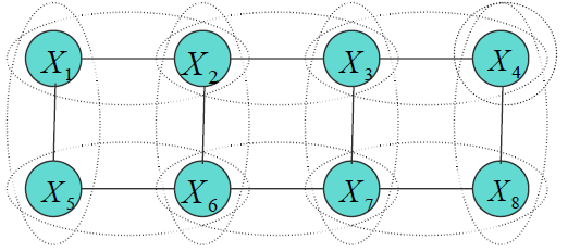
We can not write down its probability like:
\[P(X) = \frac{\prod_{\alpha} b_{\alpha}(X_{\alpha})}{\prod_{i} b_{i}^{d_i - 1}(x_i)}\]Then it’s hard to calculate the Free energy \(F(X)\). However, for a general graph, we can choose approximate \(\hat{F}(P, Q)=F_{Bethe}\), which has the formulation:
\[F_{Bethe} = \sum_{\alpha} \sum_{X_{\alpha}} b_{\alpha}(X_{\alpha}) \ln \frac{b_{\alpha}(X_{\alpha})} {f_{\alpha}(X_{\alpha})} - \sum_{i} (1-d_i) \sum_{x_i}b_i(x_i) \ln b_i(x_i) = - \langle f_{\alpha}(X_{\alpha}) \rangle - H_{Bethe}\]Note that this is equal to the exact Gibbs free energy when the factor graph is a tree, but in general, \(H_{Bethe}\) is not the same as the \(H\) of a tree.
Then for the loopy graph above, we can write the \(F_{Bethe}\) as:
\[F_{Bethe} = \sum_{(i,j) \in E}F_{ij} - \sum_i d_i F_i\]Constrained minimization of the Bethe free energy
Then we want to solve the constrained minimization problem:
We can write the Lagrange form as:
Then we can have the zero-gradient solutions:
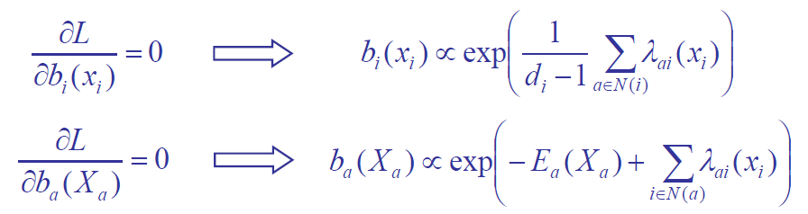
A interesting finding is that, if we identify \(\lambda_{\alpha i}(x_i) = \log(m_{i \rightarrow \alpha}(x_i)) = \log \prod_{b \in N(i) \neq \alpha} m_{b \to i}(x_i)\), then we get exactly the BP equations:
Theory of Variational Inference
We have learned two families of approximate inference algorithms: Loopy belief propagation (sum-product) and mean-field approximation. Then in this section we’ll re-exam them from a unified point of view based on the variational principle: Loop BP – outer approximation, Mean Filed – inner approximation.
Variational Methods
“Variational” is a fancy name for optimization-based formulations, which represent the quantity of interest as the solution to an optimization problem. Actually many problems can be formulated in a variational way:
-
Eigenvalue problem: find the eigenvalue \(\lambda\) of \(A\), which means \(Ax=\lambda x\) for any \(x\). Then we have the Courant-Fischer for eigenvalues: \(\lambda_{\max}(A) = \max_{||x||_{2} =1} x^T A x\).
-
Linear systems of equations: \(Ax=b, A \succ 0, x^{*} = A^{-1}b\). The variational formulation can be: \(x^{*} = \text{argmin}_x (\frac{1}{2} x^T Ax - b^Tx)\). For large systems, we can apply conjugate gradient method to compute this efficiently.
Inference Problems in Graphical Models
Given an undirected graphical model, i.e.,
\[p(x) = \frac{1}{Z} \prod_{C \in \mathcal{C}} \psi_C(x_C),\]where \(\mathcal{C}\) denotes the collection of cliques, one is interested in the inference of the marginal distributions
\[p(x_i) = \sum_{x_j, j\neq i} p(x).\]Ingredients: Exponential Families
Definition: We say \(X\) follows from an exponential family provided that the parametrized collection of density functions satisfies:
\[p(x;\theta) = \exp\left\{ \theta^T\phi(x) - A(\theta) \right\}, \qquad A(\theta)<\infty .\]Moreover, \(\phi\) is one of the sufficient statistics for \(\theta\), see Larry Wasserman’s lecture notes from 10/36-705 for more details and examples here; and \(A\) is usually known as the log partition function, which is convex and lower semi-continuous. Further,
- Parametrize Graphical Models as Exponential Family For undirected graphical model, if we assume
and let
\[A(\theta) = \log Z(\theta)\]then
\[p(x;\theta) = \exp\left( \sum_{C \in \mathcal{C}} \theta_C^T \phi(x_C)- A(\theta)\right).\]- Examples: Gaussian MRF, Discrete MRF.
Ingredients: Convex Conjugate
Definition: For a function \(f\), the convex conjugate dual, which is also known as the Legendre transform of \(f\), is defined as
\[f^* (\mu) = \sup_{\theta} \{ \theta^T\mu - f(\theta)\},\]and the convex conjugate dual is convex, no matter the original function is convex or not, and Moreover, if \(f\) is convex and lower semi-continuous, then
\[f(x) = \sup_{\mu} \{ \theta^T\mu - f^* (\mu)\}.\]- Application to Exponential Family
Let \(A\) be the log partition function for the exponential family
\[p(x;\theta) = \exp\left\{ \theta^T\phi(x) - A(\theta) \right\},\]The dual for \(A\) is
\[A^* (\mu) = \sup\{ \theta^T \mu - A(\theta): A(\theta)<\infty\},\]and the stationarity condition is,
\[\mu = \frac{\partial A(\theta)}{\partial \theta} = \mathbb{E}_{\theta} \left[ \phi(X) \right],\]we can thus represent \(\theta\) through the mean parameter \(\mu\). Therefore, we have the following Legendre mapping:
\[A^* (\mu) = \mathbb{E}_{\theta(\mu)} \left[ \log p(X;\theta(\mu)) \right] = -H(p(X;\theta(\mu))),\]where \(H\) is the Boltzmann-Shannon entropy function.
Ingredients: Convex Polytope
Half-plane Representation: the Minkowski-Weyl Theorem
Theorem: A non-empty convex polytope \(\mathcal{M}\) can be characterized by a finite collection of linear inequality constraints, i.e.
\[\mathcal{M} = \left\{ \mu: a_j^T \mu \geq b_j, j \in \mathcal{J} \right\}, \qquad |\mathcal{J}| <\infty.\]Marginal Polytope
Definition: For a distribution \(p(x)\) and a sufficient statistics \(\phi(x)\), the mean parameter is defined as:
\[\mu = \mathbb{E}_p[\phi(X)],\]and the set of all realizable mean parameters is denoted by:
\[\mathcal{M} := \left\{ \mu: \mathbb{E}_p[\phi(X)] = \mu, \text{for some distribution $p$} \right\}.\]-
\(\mathcal{M}\) is a convex set;
-
For discrete exponential families, \(\mathcal{M}\) is called the marginal polytope, and has the following convex hull representation:
By the Minkowski-Weyl Theorem, the marginal polytope can be represented by a finite collection of linear inequality constraints, see the examples for the 2-node Ising model.
Variational Principle
The exact variational formulation is:
\[A(\theta) = \text{sup}_{\mu \in \mathcal{M}} \{ \theta^T \mu - A^{*}(\mu) \},\]where \(\mathcal{M}\) is the marginal polytope, as mentioned before, which is difficult to characterize. \(A^*\) is the conjugate dual (entropy) without explicit form.
Then we’ll talk about two approximation methods: 1. mean field approximation: non-convex inner bound and exact form of entropy. 2. Bethe approximation and loopy belief propagation: polyhedral outer bound and non-convex Bethe approximation.
Mean Field Approximation
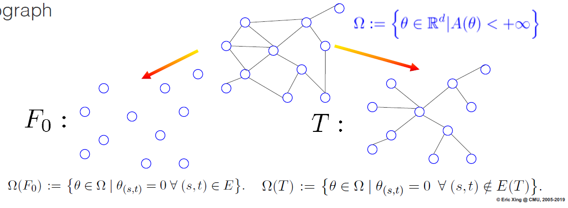
First we recall that For an exponential family with sufficient statistics \(\phi\) defined on graph \(G\), the set of realizable mean parameter set is defined as:
\[\mathcal{M}(G;\phi) = \{ \mu \in \mathbb{R}^d| \exists p \ \text{s.t.} \ E_p[\phi(X)] = \mu \}\]Then we restrict \(p\) to a subset of distributions associated with a tractable subgraph. For example, we transform a general graph with mean parameter set \(\Omega = \{ \theta \in \mathbb{R}^d | A(\theta) < +\infty \}\), to a subgraph \(F_0\) with \(\Omega(F_0) = \{ \theta \in \Omega | \theta_{(s,t)} = 0 \ \forall \ (s,t) \in E \}\), or a subgraph \(T\) with \(\Omega(T) = \{ \theta \in \Omega | \theta_{(s,t)} = 0 \ \forall \ (s,t) \in E(T) \}\). This is illustrated in the following figure.
For a given tractable subgraph \(F\), a subset of canonical parameters is:
\[\mathcal{M}(F;\phi) = \{ \tau \in \mathbb{R}^d| \tau = E_{\theta}[\phi(X)] \text{ for some } \theta \in \Omega(F) \}\]This stands for the inner approximation for variational principle. Then the mean filed method solves the relaxed problem:
\[\text{max}_{\tau \in M_F(G)} \{ \langle \tau, \theta \rangle - A_F^{*}(\tau) \}\]where \(A^{*}_F\) is the exact dual function restricted to \(M_F(G)\).
Geometry of Mean Field
Mean field optimization is always non-convex for any exponential family in which the state space \(\mathcal{X}^m\) is finite. This can be seen very easily - the marginal polytope \(\mathcal{M}(G)\) is a convex hull and \(\mathcal{M}_F(G)\) contains all the extreme points of this polytope. This implies that \(\mathcal{M}_F(G)\) is a strict subset of \(\mathcal{M}(G)\) and is thus non-convex. For example, consider a two-node Ising model:
\[\mathcal{M}_F(G) = \left\{ \tau_1, \tau_2 \in [0, 1] \quad \text{s.t.} \, \tau_{12} = \tau_1 \tau_2 \right\}\]This has a parabolic cross section along \(\tau_1 = \tau_2\) and hence it is non-convex.
Bethe Approximation and Sum-Product
The Sum-Product/Belief Propagation algorithm is exact for trees but it is approximate for loopy graphs. It is interesting to consider how the algorithm on trees is related to the variational principle and what the algorithm is doing for graphs with cycles. In fact, it turns out that the message passing updates are a Lagrange method to solve the stationary condition of the variational formulation.
Bethe Variational Problem (BVP)
In the variational formulation \(A(\theta) = \sup_{\mu\in \mathcal{M}(G)} \{\theta^T\mu - A^*(\mu)\}\), there usually exists 2 problems: the marginal polytope \(\mathcal{M}\) is hard to characterize, and the exact entropy \(- A^*(\mu)\}\) lacks explicit form. Therefore, in BVP, we use the following 2 approximation to solve the problem:
- Substitute the marginal polytope \(\mathcal{M}(G)\) with the tree-based outer bound:
- Substitute the exact entropy \(- A^*(\mu)\}\) with the exact expression for trees:
With these two ingredients, the BVP is formulated as a simple structured problem:
\[\max_{\tau \in \mathbb{L}(G)}\{ <\theta, \tau> + \sum_{s\in V} H_s(\tau_s) - \sum_{(s,t)\in E}I_{st}(\tau_{st}) \}.\]Geometry of BVP
-
Loopy BP can be derived as am iterative method for solving a Lagrangian formulation of the BVP; similar proof as for tree graphs;
-
A set of pseudo-marginals given by Loopy BP fixed point in any graph if and only if they are local stationary points of BVP;
-
For any graph, \(\mathcal{M}(G)\subset \mathbb{L}(G)\); \(\mathcal{M}(G)=\mathbb{L}(G)\) if and only if the graph is a tree;
-
For any element of outer bound \(\mathbb{L}(G)\), it is possible to construct a distribution with it as a BP fixed point.
Remark
The connection between Loopy BP and the Lagrangian formulation of the Bethe Variational Problem provides a principled basis for applying the sum product algorithm for loopy graphs. However, there are no guarantees on the convergence of the BP algorithm on loopy graphs, although there is always a fixed point of loopy BP. Even if the algorithm converges in the end, due to the non-convexity of Bethe Variational Problem, there are no guarantees on the global optimum. In general, there are no guarantees that \(A_{\text{Bethe}}(\theta)\) is a lower bound of \(A(\theta)\).
Nevertheless, the connection and understanding of this suggest a number of avenues for improving upon the ordinary sum-product algorithm, via progressively better approximations to the entropy function and outer bounds on the marginal polytope such as Kikuchi clustering
Summary
Variational methods turn the inference problem into an optimization problem via exponential families and convex duality. However, the exact variational principle is usually intractable to solve and approximations are required. In a theoretical view, there are two distinct components for approximations:
- Either inner or outer bound to the marginal polytope;
- Various approximation to the entropy function.
In this lecture, we went through the theoretical guarantee behind two mainstream variational methods: Mean field and Belief Propagation. In addition, there is another storyline on Kikuchi clustering and its variants
- Mean field: non-convex inner bound and exact form of entropy;
- Belief Propagation: polyhedral outer bound and non-convex Bethe approximation;
- Kikuchi and variants : tighter polyhedral outer bounds and better entropy approximations.
More information on this topic can be found in Section 3 and 4 from Wainwright & Jordan’s paper