Lecture 13: Approximate Inference: Monte Carlo and Sequential Monte Carlo Methods

Wrapping up variational inference, and overview of Monte Carlo methods.

Recap of Variational Principles

Last class, we reformulated probabilistic inference as an optimization problem. Invoking conjugate duality, we defined the exact variational formulation for the partition function

\[A(\theta) = \sup_{\mu \in \mathcal{M}}\left\{ \theta^T \mu - A^*(\mu) \right\}\]

where:

$\theta$ are the canonical parameters in an exponential family distribution
$\mu$ are the mean parameters
$\mathcal{M}$ is the marginal polytope (convex combination of the marginals of the sufficient statistics)
$A^*$ is the negative entropy function

Example: Two-node Ising Model

To better understand this variational formulation, we consider the two-node Ising model.

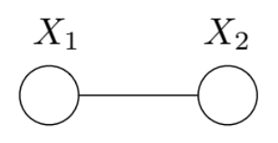
Its distribution is

\[p(x;\theta) \propto \exp\{\theta_1 x_1 + \theta_2 x_2 + \theta_{12}x_{12}\}\]

and it has sufficient statistics $\phi(x) = \left \{ x_1, x_2, x_1 x_2 \right \}$.

Plugging into the variational formulation of the partition function, we get

\[A(\theta) = \max_{\{\mu_1, \mu_2, \mu_{12}\in \mathcal{M}\}} \left\{ \theta_1 \mu_1 + \theta_2 \mu_{2} + \theta_{12} \mu_{12} - A^*(\mu) \right\}\]

where the marginal polytope $\mathcal{M}$ is defined in terms of half-spaces:

\begin{aligned} \mu_1 &\geq \mu_{12}\\ \mu_2 &\geq \mu_{12}\\ \mu_{12} &\geq 0\\ 1 + \mu_{12} &\geq \mu_1 + \mu_2 \end{aligned}

As we showed in the previous lecture, the dual $A^*$ can be computed as the negative entropy of the model:

\[A^*(\mu) = \mu_{12}\log\mu_{12} + (\mu_1 - \mu_{12})\log(\mu_1 - \mu_{12}) + (\mu_{2} - \mu_{12})\log(\mu_2 - \mu_{12}) + (1 + \mu_{12} - \mu_1 - \mu_2) \log(1 + \mu_{12} - \mu_1 - \mu_2)\]

By plugging in for $A^*$, taking the derivatives of the objective function, and setting to zero, we can solve the variational problem and arrive at the optima. For instance,

\[\mu_1(\theta) = \frac{\exp(\theta_1) + \exp(\theta_1 + \theta_2 + \theta_{12})} {1 + \exp(\theta_1) + \exp(\theta_2) + \exp(\theta_1 + \theta_2 + \theta_{12})}\]

In this example, we were able to compute everything exactly. However this is not always possible, and so approximations such as the mean field method, Bethe approximation, and loopy belief propagation are used. The mean field method (to be described more in the following section) gives a non-convex inner bound and exact form of entropy. The non-convex Bethe approximation and loopy belief propagation (discussed later in these notes) provide polyhedral outer bounds.

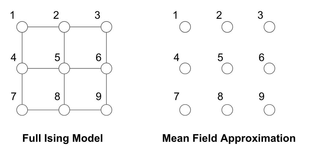
Mean Field Approximation

Graphically, the mean field approximation can be thought of as a tractable subgraph approximation $F$ to the original full graph $G$. Consider a graph with $x_i$’s for each node and canonical parameters defined on each edge. The space of these parameters $\theta$ is such that the partition function $A(\theta)$ is bounded. If there is no edge connecting two nodes $x_i$and $x_j$, that is, $\theta_{ij} = 0$, then we know that the mean parameters are related such that $\mu_{ij} = P(x_i, x_j) = P(x_i)P(x_j) = \mu_{i}\mu_{j}$.

Mean Field Methods

For a given tractable subgraph $F$, a subset of canonical parameters is

\[\mathcal{M}(F; \phi) := \{ \tau \in \mathcal{R}^d | \tau = \mathcal{E}_\theta [\phi(X)] \text{ for some } \theta \in \Omega(F)\}\]

This subset of parameters constrained by the subgraph defines a new subspace, known as the inner approximation to the full marginal polytope. That is, $\mathcal{M}(F;\phi)^o \subseteq \mathcal{M}(G;\phi)^o$.

Making the mean field approximation, we solve the relaxed problem

\max_{\tau \in \mathcal{M}_F(G)}\left \{\left \langle \tau, \theta \right \rangle - A_F^*(\tau) \}\right \}

where $A_F^* = A^* \lvert_{\mathcal{M}_F (G)}$ is the exact dual function restricted to $\mathcal{M}_F(G)$.

Naive Mean Field for Ising Model

Consider the Ising model in its $\{ 0, 1\}$ representation:

\[p(x) \propto \exp\left\{ \sum_{s\in V}{x_s \theta_s} + \sum_{(s,t)\in E}{x_s x_t \theta_{st}} \right\}\]

In making the mean field approximation, we cut out all of the edges as shown below:

The mean parameters are:

\[\begin{aligned} \mu_s &= \mathbb{E}_p [X_s] = P(X_s = 1) & \forall s \in V \\ \mu_{st} &= \mathbb{E}_p [X_s X_t] = P[(X_s, X_t) = (1,1)] & \forall (s, t) \in E \end{aligned}\]

For the fully disconnected graph $F$,

\[\mathcal{M}_F(G) = \left\{ \tau \in \mathbb{R}^{|V| + |E|} | 0 \leq \tau_s \leq 1, \forall s \in V, \tau_{st} = \tau_s \tau_t, \forall (s,t) \in E \right\}\]

Note that by the mean field approximation, we have that $\tau_{st} = \tau_s \tau_t$. The dual decomposes into a sum, one term for each node:

\[A_F^*(\tau) = \sum_{s \in V}[\tau_s \log \tau_s + (1-\tau_s) \log(1 - \tau_s)]\]

The mean field objective, which lower bounds $A(\theta)$, is as stated below.

\[A(\theta) \geq \max_{(\tau_1, ..., \tau_m) \in [0,1]^m} \left\{ \sum_{s \in V}{\theta_s \tau_s} + \sum_{(s,t) \in E}{\theta{st}\tau_s\tau_t - A_F^*(\tau)} \right\}\]

To solve, take the derivative with respect to $\tau$ to arrive at the naive mean field update equations:

\[\tau \leftarrow \sigma\left ( \theta_s + \sum_{t \in N(s)} \theta_s \tau_t \right )\]

Summary of Mean Field Approximation

Mean field optimization is always non-convex for any exponential family in which the state space $\mathcal{X}^m$ is finite. Thus, it is not guaranteed to get the global optimum.
Recall that the marginal polytope is a convex hull, and that the adjusted marginal under the mean field approximation contains all the extreme points. Note that if this adjusted marginal is a strict subset, then it must be non-convex.
Simple algorithm, but solves a much more complex intractable problem in an iterative fashion.

Bethe Approximation and Sum-Product

Sum-Product Algorithm Recap

Message passing rule:

\[M_{ts}(x_s) \leftarrow \kappa\sum_{x_t'} \bigg\{ \psi_{st}(x_s, x_t')\psi_t(x_t')\prod_{u\in N(t)/s}M_{ut}(x_t') \bigg\}\]

Marginals:

\[\mu_{s}(x_s) = \kappa \psi_{s}(x_s)\prod_{t\in N(s)}M^{*}_{ts}(x_s)\]

Trees Graphic Models

We have discrete variables $X_s \in {0, 1, …, m_s - 1}$ on a tree $T = (V, E)$.

The sufficient statistics are:

$\mathbb{I}_j(x_s) $ where $s \in V, j \in \chi_s$
$\mathbb{I}_{jk}(x_s, x_t)$ where $(s, t)\in E, (j, k)\in \chi_s \times \chi_t$

Then the mean parameters are marginals and pair-wise marginals:

\[\mu_s(x_s) = \mathbb{P}(X_s=x), \ \mu_{st}(x_s, x_t) = \mathbb{P}(X_s=x_s, X_t=x_t)\]

Marginal Polytopes for Trees

The algorithm produces an exact solution for tree graphic models. The marginal polytope for is the same as the true polytope, because the local consistency is sufficient for global consistency in a tree.

\[\mathcal{M}(T) = \bigg\{ \mu \ge 0 | \sum_{x_s}\mu(x_s) = 1, \sum_{x_t}\mu_{st}(x_s, x_t) = \mu(x_s) \bigg\}\]

If $\mu \in \mathcal{M}(T)$, then

\[p_\mu(x):=\prod_{s\in V}\mu_s(x_s)\prod_{(s, t)\in E} \frac{\mu_{st}(x_s, x_t)}{\mu_s(x_s)\mu_t(x_t)}\]

Decomposition of Entropy for Trees

In order to perform optimization, we define $A^*(\mu) = - H(p(x;\mu))$.

The entropy can be decomposed as:

\begin{aligned} H(p(x;\mu)) & = - \sum_xp(x;\mu) \log p(x;\mu) \\ &= \sum_{s\in V}\bigg(-\sum_{x_s}\mu_s(x_s)\log\mu_s(x_s)\bigg) + \sum_{(s, t)\in E}\bigg( -\sum_{x_s, x_t}\mu_{st}(x_s, x_t)\log\frac{\mu_{st}(x_s, x_t)}{\mu_s(x_s)\mu_t(x_t)} \bigg) \\ &= \sum_{s\in V}H_s(\mu_s) - \sum_{(s, t)\in E}I_{st}(\mu_{st})\\ \end{aligned}

Exact Variational Inference on Trees

With $\mu$ as local parameters satisfying both local and global consistency, consider the following problem:

\[\begin{aligned} A(\theta) &= \max_{\mu \in \mathcal{M}(T)} \bigg\{ \langle \theta ,\mu \rangle - A^*(\mu)\bigg\} \\ &= \max_{\mu \in \mathcal{M}(T)} \bigg\{ \langle \theta ,\mu \rangle +\sum_{s\in V}H_s(\mu_s) -\sum_{(s, t)\in E}I_{st}(\mu_{st}) \bigg\} \end{aligned}\]

We use the Lagrangian to solve the problem:

\[\mathcal{L}(\mu, \lambda) = \langle \theta, \mu \rangle + \sum_{s\in V}H_s(\mu_s) -\sum_{(s, t)\in E}I_{st}(\mu_{st})\]

We assign Lagrange multipliers:

$\lambda_{ss}$ for $C_{ss}(\mu) := 1 - \sum_{x_s}\mu(x_s) = 0$,
$\lambda_{ts}(x_s)$ for $C_{ts}(x_s;\mu) := \mu(x_s) - \sum_{x_t}\mu_{st}(x_s, x_t) = 0$

The derivatives are given by

\[\begin{aligned} \frac{\delta\mathcal{L}}{\delta\mu_s(x_s)} &= \theta_s(x_s) - \log\mu_s(x_s) + \sum_{t \in N(s)} \lambda_{ts}(x_s) + C \\ \frac{\delta\mathcal{L}}{\delta\mu_{st}(x_s, x_t)} &= \theta_st(x_s, x_t) - \log \frac{\mu_{st}(x_s, x_t)}{\mu_s(x_s)\mu_t(x_t)} - \lambda_{ts}(x_s) - \lambda_{st}(x_t) + C' \end{aligned}\]

By setting the derivatives to 0 and solving for $\mu$, we get:

\[\begin{aligned} \mu_s(x_s) &\propto \exp\{\theta_s(x_s)\}\prod_{t\in N(s)}\exp\{\lambda_{ts}(x_s)\} \\ \mu_s(x_s, x_t) &\propto \exp\{\theta_s(x_s)+ \theta_t(x_t) + \theta_{st}(x_s, x_t)\}\prod_{u\in N(s)/t}\exp\{\lambda_{us}(x_s)\}\prod_{v\in N(t)/s}\exp\{\lambda_{vs}(x_t)\}\\ \end{aligned}\]

After adjusting the Lagrange multipliers to enforce constraints, $\mu$ correspond to cluster message and singleton message. We conclude that the message passing updates are a Lagrange method to solve the stationary condition of the variational formulation.

\[M_{ts}(x_s) \leftarrow \sum_{x_t} \exp\{\theta_t(x_t) + \theta_{st}(x_s, x_t)\}\prod_{u\in N(t)/s}M_{ut}(x_t)\]

Belief Propagation on Arbitrary Graphs and Bethe Approximation

Inspired by sum-product algorithm on tree graph, we can have another approximation approach to solve the variational formulation:

\[A(\theta)=\sup_{\mu\in \mathcal{M}}\{\theta^T\mu-A^*(\mu)\}\]

The two main difficulties of above variational problem are:

The marginal polytope $\mathcal{M}$ is hard to characterize.
The exact entropy $-A^*(\mu)$ lacks explicit form.

To address the first difficulty, we use the tree-based outer bounder:

\mathcal{L}(G) = \left \{ \tau\geq 0 | \sum_{x_s} \tau_s(x_s)=1,\sum_{x_t}\tau_{st}(x_s,x_t)=\tau_s(x_s)\right \}

The conditions on the $\tau$ are the locally consistent conditions, and we don’t care about whether they are globally consistent or not. There are some other global constraint for general graphs. So, $\mathcal{L}(G)\supseteq\mathcal{M}(G)$, which means that it is an outer bounder. Since the number of faces of $\mathcal{L}(G)$ grows linearly with the size of the graph, it is easier to characterize.

For the second difficulty, we can approximate the true entropy with Bethe entropy, which is the exact expression for trees:

\[-A^*(\tau)\approx H_{Bethe}(\tau):=\sum_{s\in V} H_s(\tau_s)-\sum_{(s,t)\in E}I_{st}(\tau_{st})\]

It has the explicit form, which is the sum of entropy of every node minus the sum of mutual information of every edge.

Combining these two approximations, we derive the Bethe Variational Problem (BVP):

\[A_{Bethe}(\theta)= \sup_{\tau\in \mathcal{L}(G)}\{\theta^T\tau +\sum_{s\in V} H_s(\tau_s)-\sum_{(s,t)\in E}I_{st}(\tau_{st})\}\]

In contrast to the Mean Field Method, which uses an inner approximation $\mathcal{M}_F(G)$ for $\mathcal{M}(G)$ and the exact dual function on $\mathcal{M}_F(G)$, the BVP uses an outer bounder $\mathcal{L}(G)$ for the marginal polytope and an approximated entropy. If the graph is a tree, the two approximations above are actually exact, so the BVP are exact for trees.

Some notes about BVP:

It may not converge (because the objective function is not convex).
It may not converge to the right answer (because the solution may not be in the $\mathcal{M}(G)$).
There is no guarantee that $A_{Bethe}(\theta)$ is the lower bound of $A(\theta)$

In summary:

Variational methods in general turn inference into an optimization problem via exponential families and convex duality.
The exact variational principle is intractable to solve. There are two distinct components for approximation:
1. Inner or outer bound for the marginal polytope
2. Various approximation for the entropy function
Three approximated approaches:
1. Mean field: non-convex inner bound of marginal polytope and exact form of entropy
2. Bethe Variational Problem: polyhedral outer bound and non-convex Bethe approximation of entropy.
3. Kikuchi: tighter polyhedral outer bounds and better entropy. approximations

Monte Carlo and Sequential Monte Carlo Methods

Overview

Changing gears, we now introduce an alternative set of methods for approximate inference. These methods are based on on stochastic simulation/sampling from a target distribution. In many inference tasks (such as finding a marginal $P(x)$, computing the partition function $A(\theta)$, or finding the expectation of an arbitrary function), we are interested in quantities that in a sense sum over the configurations of a true distribution.

\[E_p(f(x)) = \int f(x)p(x)dx\]

In such problems, we may not have the true distribution in closed-form or this integral might be tough to carry out. However, if we are able to simply sample from this distribution, approximate inference is possible by using a sample-based representation of $p(x)$. Here, the true distribution is now represented by the collection of $N$ samples that we draw and we can rephrase the problem as

\[E_p(f(x)) = \frac{\sum f(x^n)}{N}\]

This is in essence the spirit of Monte Carlo Methods, which give us a stochastic representation of a potentially complex distribution. This representation can then be used to compute the marginals and expectations that we care about. The good news is that these approximations are asymptotically exact (they get closer to the true $E[f(x)]$ as $N \rightarrow \infty)$ and are flexible for any distribution. However, there are key non-trivial challenges that must be overcome:

How exactly do we draw from them from complex distributions?
Not all samples are equally useful (more on this later).
How do we know we’ve drawn enough samples?

Direct Sampling: A Naive Approach

We first discuss a seemingly obvious solution for sampling in the case where we can easily sample from the joint distribution. Such a case is if we have a BN, which gives us a straightforward generative model for a set of RVs. To sample from a joint distribution, we can simply traverse a BN in topological order, constructing our sample by filling in values node by node. At each step, we use the CPDs as well as the previously filled-in values. We can run this process many times and then use frequency counts to perform any inference task, such as finding a conditional probability.

However, we observe that we run into an issue when we deal with large models and want to consider rare events. In such cases our approximate inference estimates can easily be biased because as the sample size is too small. If we want to condition on such a rare event, our frequency counts will give a very low-sample estimate. In the worst case, we may even have 0 examples for a particular rare event, falsely indicating that such events are impossible and also making it impossible to condition on such events. This can be extended in general to any case where we can sample from the joint easily. If we want inferences that involve conditionals, we will have to perform and keep track of an exceedingly large number of samples.

Rejection Sampling

Direct sampling assumed the joint was easy to sample from. However, now let’s consider a case where

The target distribution $p(x)$ is difficult to sample from.
The unnormalized distribution $\tilde{p}(x) = \frac{1}{Z}p(x)$ is easy to evaluate. Note that this alone does not make $p(x)$ amenable to sampling.
The proposal distribution $q(x)$ is a distribution that we can easily sample from (e.g., uniform or normal).
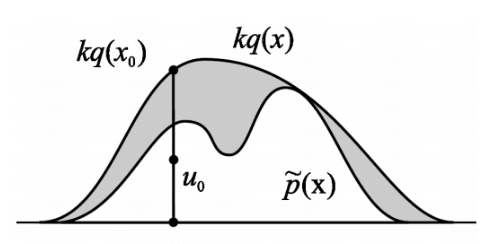
$k$ is a chosen constant such that $kq(x) \geq \tilde{p}(x)$ for all $x$. This is called the comparison function.

Procedure

Sample $x_0$ from $q(x).$
Sample a number $u_0$ from the uniform distribution over $[0,kq(x_0)]$.
Reject the sample if $u_0 > \tilde{p}(x_0)$ and retain the sample otherwise.

Note that steps 2 and 3 are akin to accepting the sample $x_0$ with probability $\frac{\tilde{p}(x_0)}{kq(x_0)}$. Pictorially for a univariate case, this process is akin to sampling uniformly any point in the area under the $kq(x)$ curve and accepting only if it does not land in the gray region.

Correctness

We can formally show that this procedure samples correctly from $p(x)$. First we observe that the procedure selects a particular $x$ with density proportional to $q(x) \cdot \frac{\tilde{p}(x)}{kq(x)}$. Then, the sampling mechanism generates samples according to a distribution $p_s(x)$ which is equal to

\begin{aligned} p_s(x) &= \frac{q(x)\frac{\tilde{p}(x)}{kq(x)}}{\int q(x)\frac{\tilde{p}(x)}{kq(x)} dx} \\ &= \frac{ \frac{\tilde{p}(x)}{kq(x)}}{\int \frac{\tilde{p}(x)}{kq(x)}dx} \\ &= \frac{\tilde{p}(x)}{\int\tilde{p}(x)}\\ &= p(x) \end{aligned}

Pitfalls

If the proposal distribution $q(x)$ is not chosen well (i.e., differs greatly from $p(x)$), then even an optimally chosen $k$ can result in a huge rejection region. This implies a large waste of samples that will be rejected. Even if distributions seem similar, in higher dimensions this rejection volume can be very high. In class we discussed the example where using $d$-dimensional gaussians

\[\begin{aligned} Q &\sim N(\mu, \sigma_q^{2/d} ) \\ P &\sim N(\mu, \sigma_p^{2/d} ) \end{aligned}\]

for $d = 1000$ and $\sigma_q$ only 1 percent bigger than $\sigma_p$ results in an acceptance rate of only $\approx \frac{1}{20000}$.

One potential way to fix this is to use adaptive rejection sampling, which covers $\tilde{p}$ with an envelope of piecewise functions instead of one proposal distribution $q$ but this gets rather complicated.

Importance Sampling

Suppose we want to evaluate expectations using samples from a complicated probability distribution. We assume that:

$p(x)$ is hard to sample from but easy to evaluate
$q(x)$ is easy to sample from
$f(x)$ is a function we want to evaluate in expectation: $\langle f(x) \rangle$.
$q(x) > 0$ whenever $p(x)>0$ or $q$ dominates $p$.

Unnormalized Importance Sampling

Procedure:

Draw $M$ samples $x^{(m)}$ from $q(x)$.
Determine weights $w^{(m)}$ for samples equal to the likelihood ratio $w^{(m)} = \frac{p(x^{(m)})}{q(x^{(m)})}$.
Compute expectation as:

\[\langle f(x) \rangle = \frac{1}{M} \sum_m f(x^m) w^m\]

We call this unnormalized because these weights are likelihood ratios, so there is no reason that they need to sum to $1$. However, it gives us a first approximation to the true distribution.

Correctness

Note that this does not give us sample from the target distribution but we can prove correctness for the expected value estimate.

\begin{aligned} \langle f(x) \rangle &= \int f(x)p(x)dx \\ &= \int f(x)\frac{p(x)}{q(x)}q(x)dx \\ &\approx \frac{1}{M} \sum_m f(x^m)\frac{p(x^m)}{q(x^m)} \\ &= \frac{1}{M} \sum_m f(x^m)w^m \end{aligned}

The key step is the third equality where we can approximate the integral assuming $x^m$ are drawn from $q(x)$ which they actually are in the procedure.

Normalized Importance Sampling

Here we no longer assume that we know $p(x)$ and instead only know it up to a constant factor $\tilde{p}(x) = \alpha p(x)$. This is a common situation, such as when we want a conditional probability when we know the joint $P(x,e)$ but not the marginal $P(e)$. In this situation we can do the following.

Procedure

Draw $M$ samples $x^{(m)}$ from $q(x)$.
Calculate ratios $r^{(m)}$ for samples equal to $r^{(m)} = \frac{\tilde{p}(x^{(m)})}{q(x^{(m)})}$.
Compute expectation as

\[\langle f(x) \rangle = \frac{\sum_m f(x^m)r^m}{\sum_m r^m}\]

Correctness

We observe first that

\begin{aligned} \langle r(x) \rangle_q &= \int \frac{\tilde{p}(x)}{q(x)}q(x)dx \\ &= \int \tilde{p}(x)dx \\ &= \alpha \end{aligned}

\begin{aligned} \langle f(x) \rangle &= \int f(x)p(x)dx \\ &= \frac{1}{\alpha}\int f(x)\frac{\tilde{p}(x)}{q(x)}q(x)dx \\ &= \frac{\int f(x)r(x)q(x)dx}{\int r(x)q(x)dx} \\ &\approx \frac{\sum_m f(x^m)r^m}{\sum_m r^m} \\ &= \sum_m f(x^m)w^m \end{aligned}

Again the key step is the fourth equality were we approximate both numerator and denominator using samples drawn form $q(x)$. Here we observe that $\sum_m w^m = 1$, hence why we call it the normalized version. The key takeaway is that we don’t need to know the normalization constant for the target distribution.

Comparison between Normalized and Unnormalized

On finite samples. The unnormalized version gives an unbiased estimator of the true expectation while the normalized version gives a biased estimator of the true expectation. However, the variance of the normalized version is generally lower in practice.

Pitfalls

These importance sampling approaches are based on likelihood weighting, which is simple to operate but still might be inaccurate in some peculiar scenarios. Again the core issue is when our proposal and target distributions are not similar enough. Consider the following

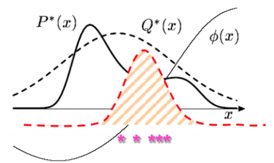
Essentially, what importance sampling is trying to do is to weight the samples such that they reflect relative importance to each other. The hope is that even if regions where $P$ has high density are low probability regions in $Q$, the weighting on these samples will be high enough to offset the fact we won’t see many samples in this region. Similar to the arguments against direct sampling, if $Q$ has really thin tails where $P$ has high probability (and where the means are going to actually be located around), we may simply never see enough samples from this region. We might need an extraordinary number of samples to offset this, meaning most of our samples are wasteful as they are very low importance. In terms of a sampling algorithm, this is compounded by the fact that usually the stopping condition is when the estimate for the mean of $f(x)$ starts to converge. However, in the scenario we described, its possible to have a stable estimate even if all the samples are coming from low probability regions of $P$. Thus, the algorithm will stop even though the mean estimate is very inaccurate. There are a couple of potential solutions to this problem.

We could use heavy-tailed proposal distributions. However, this has the disadvantage of inefficiently drawing a lot of wasted samples with low importance.
We can use weighted re-sampling (see next section).

Weighted Re-Sampling

Draw $N$ samples from $q$: $X_1, …, X_N$
Construct weights $w_1, …, w_N$ equal to $w^m = \frac{P(X^m)/Q(X^m)}{\sum_m P(X^m)/Q(X^m)} = \frac{r^m}{\sum_m r^m}$
Sub-Sample $N’$ examples $x$ from ${X_1, …, X_N}$ with probability ${w_1, …, w_N}$ with usually $N’ > > N$.

This is a sense amplifies the high importance samples while diminishes the low importance samples.

Particle Filters Sketch

Here is another algorithm that uses the re-sampling idea to do very efficient and elegant sequential inference tasks. The goal here is to make a fast sampling based inference algorithm for the state space model we looked at previously.

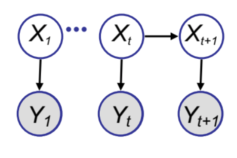
We have already studied the Kalman Filter algorithm for this model. However, KF is often demanding to implement in high dimensional spaces or when the transitional model is not Gaussian. Hence, a sampling algorithm could be useful. The goal here is to get samples from the posterior $p(X_t | Y_{1:t})$ using the weighted re-sampling approach.

We establish a recursive relation like we did for the KF algorithm. We want to update the posterior distribution of the hidden variables in light of each new observation. This is essentially a recursive two step process:

The starting point at time $t$ is $p(X_t \| Y_{1:t}) = p(X_t \| Y_t, Y_{1:t-1}) = \frac{p(X_t \| Y_{1:t-1})p(Y_t \| X_t)}{\int p(X_t \| Y_{1:t-1})p(Y_t \| X_t)dX_t}.$
We want to draw samples from $p(X_t | Y_{1:t-1})$ (treat like our proposal distribution for $p(X_t | Y_{1:t})$) and give them weights equal to $w_t^m = \frac{p(Y_t | X_t^m)}{\sum_{m=1}^M p(Y_t | X_t^m)} $. We can now represent $p(X_t | Y_{1:t})$ as the set of samples and weights, noting that $\sum_m w_t^m = 1$.
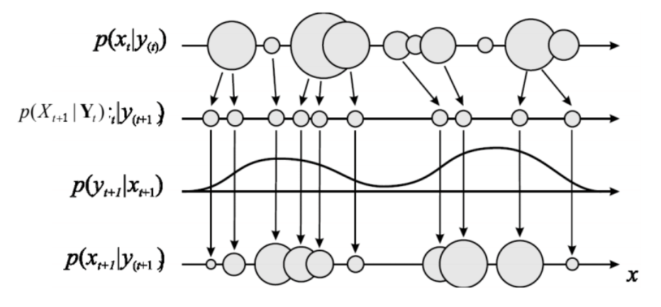
To find weights and samples at the next time step for $p(X_{t+1} | Y_{1:t+1})$, we do a time update and then a measurement update:

Time update: We decompose the probability into a term that we can replace with our sample representation and the transition probability:

\[p(X_{t+1} \| Y_{1:t}) = \int p(X_t+1 \| X) p(X_t \| Y_{1:t})dx \approx \sum_m w_t^m p(X_{t+1} \| X_t^{(m)})\]

The final term is the weighted sum of the transition probabilities conditioning on the samples of the previous states. This is a mixture distribution and samples can be easily drawn by choosing a component $m$ with probability $w^m$ and then drawing a sample from the relevant component. We again draw a set of samples and corresponding weights.

Measurement Update: Here we essentially perform step 1 again except now using the sample representation generated in the Time Update. We have a new observation $Y_{t+1}$ which we use to generate new weights for the Time Update in the next step.

Trading the Time and Measurement updates, we can proceed sequentially down the chain. The following schematic illustrates the process where the mixture distribution for the posterior at each time step is represented by circles whose sizes indicate their weights.

Particle Filters are especially interesting because we can now draw samples from more complicated distributions such as SSMs.

Rao-Blackwellised Sampling

The idea of Rao-Blackwellised Sampling is that if our samples involve a long list of RVs, we will get high variance in any estimates we make. However, we can sample a smaller subset $X_p$ if we know that conditional on this subset, the expectation on the rest of the RVs can be computed analytically. We can show this results in a lower variance estimate.

\begin{aligned} E_{p(X|e)}[f(X)] &= \int p(x_p, x_d | e) f(x_p, x_d) dx_pdx_d \\ &= \int_{x_p} p(x_p | e) \left(\int_{x_d} p(x_d | x_p, e)f(x_p,x_d)dx_d \right) dx_p\\ &= \int_{x_p} p(x_p | e) E_{p(X_d|x_p,e)}[f(x_p,x_d)dx_d] dx_p\\ &= \frac{1}{M} \sum_m E_{p(X_d|x_p^m,e)}[f(x_p^m,x_d)dx_d] \end{aligned}

where the $x_p^m \sim p(x_p | e)$.

Using law of total variance

\[\text{Var}[\tau(X_p, X_d)] = \text{Var}[E[\tau(X_p, X_d)|X_p]] + E[\text{Var}[\tau(X_p, X_d)|X_p]]\]

we get

\[\text{Var}[E[\tau(X_p, X_d)|X_p]] \leq \text{Var}[\tau(X_p, X_d)]\]

which implies that $\tau(X_p, X_d) = E[f(X_p,X_d) \lvert X_p]$ has lower variance.