Lecture 14: Approximate Inference: Markov Chain Monte Carlo

An introduction of Markov Chain Monte Carlo methods.

Recap of Monte Carlo

Monte Carlo methods are algorithms that:

• Generate samples from a given probability distribution $p(x)$.
• Estimate expectations of functions $E[f(x)]$ under a distribution $p(x)$.

Why is Monte Carlo useful?

• Can use samples of $p(x)$ to approximate $p(x)$ itself
  • Allow us to do graphical model inference when we can’t compute $p(x)$.
• Expectations $E[f(x)]$ reveal interesting properties about $p(x)$, e.g., means and variances.

Limitations of Monte Carlo

• Direct sampling
  • Hard to get rare events in high-dimensional spaces.
  • Infeasible for MRFs, unless we know the normalizer $Z$.
• Rejection sampling, Importance sampling
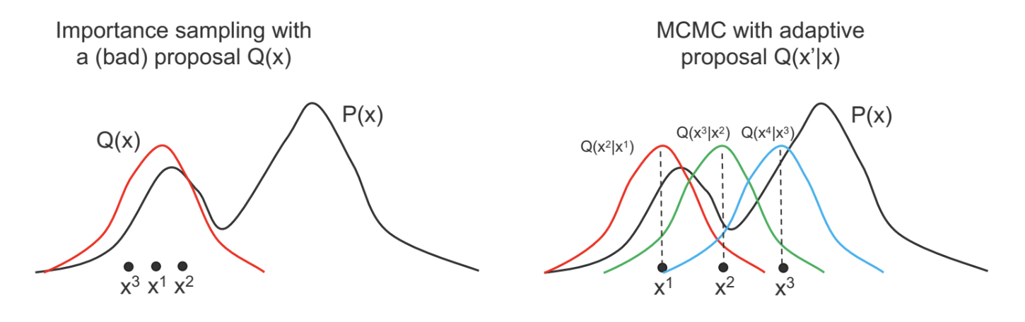
  • Do not work well if the proposal $Q(x)$ is very different from $P(x)$.
  • Yet constructing a $Q(x)$ similar to $P(x)$ can be difficult.
    • Requires knowledge of the analytical form of $P(x)$ - but if we had that, we wouldn’t even need to sample!
• Intuition: Instead of a fixed proposal $Q(x)$, use an adaptive proposal.

Markov Chain Monte Carlo (MCMC)

MCMC algorithms feature adaptive proposals.

• Instead of $Q(x^\prime)$, use $Q(x^\prime \mid x)$ where $x^\prime$ is the new state being sampled, and $x$ is the previous sample.
• As $x$ changes, $Q(x^\prime \mid x)$ can also change (as a function of $x^\prime$).

Comparison between using a fixed (bad) proposal and an adaptive proposal.

To understand how MCMC works, we need to look at Markov Chains first.

Markov Chains

• A Markov Chain is a sequence of random variables $x^{(1)}$, $x^{(2)}$, …, $x^{(n)}$ with the Markov Property

\(P(x^{(n)}=x\ |x^{(1)}, ..., x^{(n-1)})=P(x^{(n)}=x\ |x^{(n-1)})\)

• $P(x^{(n)}=x\mid x^{(n-1)})$ is known as the transition kernel.
• The next state depends only on the preceding state.
• Random variables $x^{(i)}$ can be vectors.
  • We define $x^{(i)}$ to be the t-th sample of all variables in a graphical model
  • $x^{(i)}$ represents the entire state of the graphical model at time $t$.
• We study homogeneous Markov Chains, in which the transition kernel $P(x^{(n)}=x\mid x^{(n-1)})$ is fixed with time.
  • To emphasize this, we will call the kernel $T(x^\prime\mid x)$, where $x$ is the previous state and $x^\prime$ is the next state.

Markov Chains Concepts

Define a few important concepts of Markov Chains(MC)

• Probability distribution over states: $\pi^{(t)}(x)$ is a distribution over the state of the system $x$, at time $t$.
  • When dealing with MCs, we don’t think of the system as being in one state, but as having a distribution over states.
  • For graphical models, remember that $x$ represents all variables.
• Transitions: recall that states transition from $x^{(t)}$ to $x^{(t+1)}$ according to the transition kernel $T(x^\prime\mid x)$.
  • We can also transition entire distributions: \(\pi^{(t+1)}(x')=\sum_{x} \pi^{(t)}(x)T(x' \mid x)\)
  • At time t, state $x$ has probability mass $\pi^{(t)}(x)$. The transition probability redistributes this mass to other states $x^\prime$.
• Stationary distributions: $\pi^{(t)}(x)$ is stationary if it does not change under the transition kernel: $\pi(x^\prime)=\sum_{x} \pi(x)T(x^\prime\mid x)$, for all $x^\prime$. To understand stationary distributions, we need to define some notions:
  • Irreducible: an MC is irreducible if you can get from any state $x$ to any other state $x^\prime$ with probability > 0 in a finite number of steps, i.e., there are no unreachabble parts of the state space.
  • Aperiodic: an MC is aperiodic if you can return to any state $x$ at any time.
    • Periodic MCs have states that need ≥2 time steps to return to (cycles).
  • Ergodic (or regular): an MC is ergodic if it is irreducible and aperiodic
    • Ergodicity is important: it implies you can reach the stationary distribution $\pi_{st}(x)$, no matter the initial distribution $\pi^{(0)}(x)$.
    • All good MCMC algorithms must satisfy ergodicity, so that you can’t initialize in a way that will never converge.
  • Reversible (detailed balance): an MC is reversible if there exists a distribution $\pi(x)$ such that the detailed balance condition is satisfied: \(\pi(x')T(x\ |x')=\pi(x)T(x'\ |x)\) Probability of $x^\prime \rightarrow x$ is the same as $x\rightarrow x^\prime$.
    • Reversible MCs always have a stationary distribution! Proof:
    \begin{aligned} \pi(x')T(x\ |x') & = \pi(x)T(x'\ | x) \\ \sum_{x}\pi(x')T(x\ |x') & = \sum_{x}\pi(x)T(x'\ | x) \\ \pi(x')\sum_{x}T(x\ |x') & = \sum_{x}\pi(x)T(x'\ | x) \\ \pi(x') & = \sum_{x}\pi(x)T(x'\ | x) \end{aligned}

    Note that the last line is the definition of a stationary distribution!

Metropolis-Hastings (MH) – An MCMC method

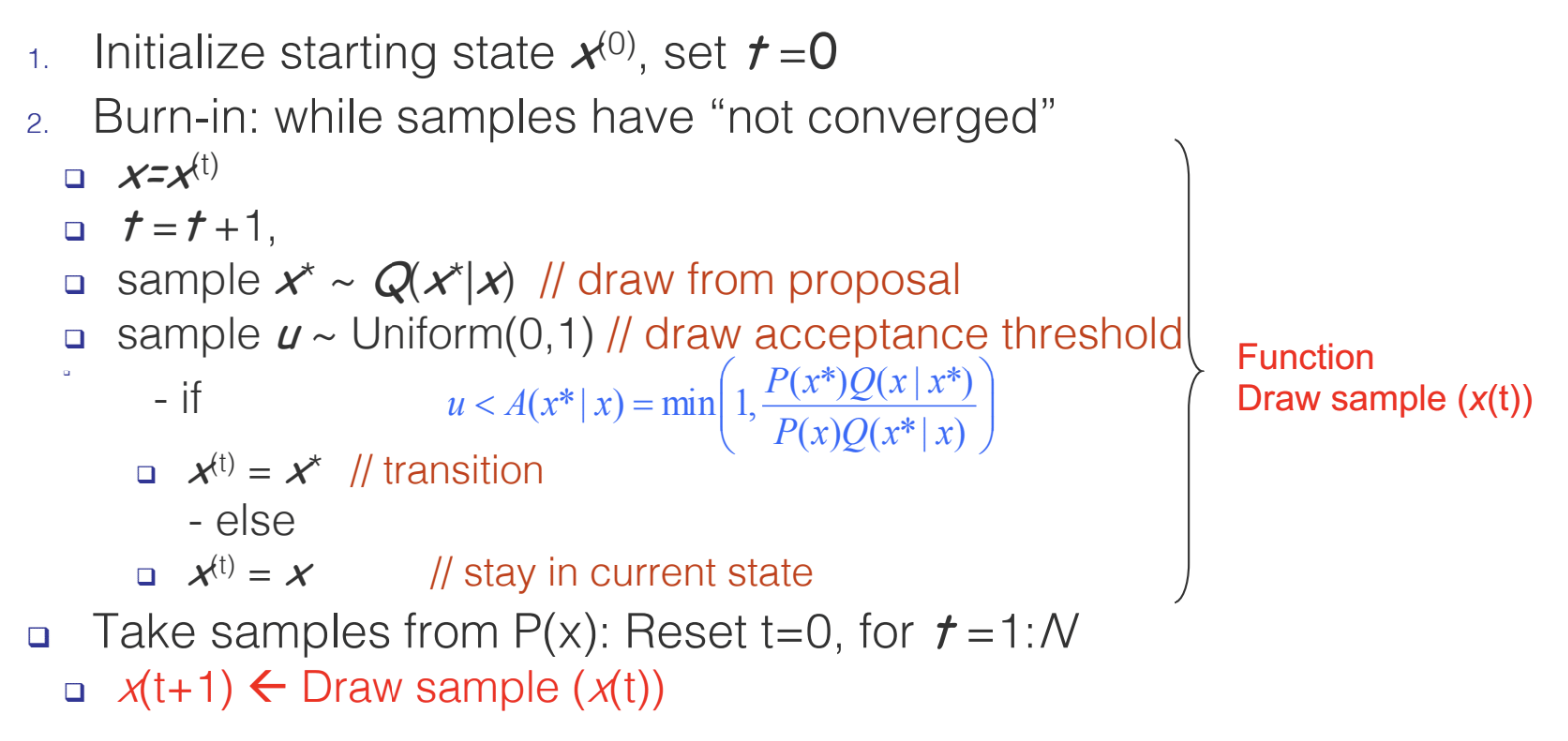
How the MH algorithm works in practice

1. Draws a sample $x^\prime$ from $Q(x^\prime\mid x)$, where x is the previous sample.
2. The new sample $x^\prime$ is accepted with some probability $A(x^\prime \mid x)=min(1, \frac{P(x^\prime)Q(x\mid x^\prime)}{P(x)Q(x^\prime\mid x)})$
   • $A(x^\prime\mid x)$ is like a ratio of importance sampling weights
   • $P(x^\prime)/Q(x^\prime\mid x)$ is the importance weight for $x^\prime$, $P(x)/Q(x\mid x^\prime)$ is the importance weight for $x$.
   • We devide the importance wieght for $x^\prime$ by that of $x$.
   • Notice that we only need to compute $P(x^\prime)/P(x)$ rather than $P(x^\prime)$ or $P(x)$ separately, so we don’t need to know the normalizer.
   • $A(x^\prime\mid x)$ ensures that, after sufficiently many draws, our samples will come from the true distribution $P(x)$.

The Metropolis-Hastings Algorithm

Why does Metropolis-Hastings work?

Since we draw a sample $x^\prime$ according to $Q(x^\prime\mid x)$, and then accept/reject according to $A(x^\prime\mid x)$, the transition kernel is: \(T(x'\mid x)=Q(x'\mid x)A(x'\mid x)\)

We can prove that MH satisfies detailed balance (or reversibility):

Recall that $A(x^\prime\mid x)=min(1, \frac{P(x^\prime)Q(x\mid x^\prime)}{P(x)Q(x^\prime\mid x)})$, which implies the following:

\[\text{If } A(x^\prime\mid x)<1 \text{ then } \frac{P(x^\prime)Q(x\mid x^\prime)}{P(x)Q(x^\prime\mid x)}>1 \text{ and thus } A(x\mid x^\prime)=1\]

Now suppose $A(x^\prime \mid x)<1$ and $A(x \mid x^\prime)=1$. We have:

\begin{aligned} A(x'\ |x) & = \frac{P(x')Q(x\ |x')}{P(x)Q(x'\ |x)} \\ P(x)Q(x'\ |x)A(x'\ |x) & = P(x')Q(x\ |x') \\ P(x)Q(x'\ |x)A(x'\ |x) & =P(x')Q(x\ |x')A(x\ |x') \\ \pi(x')T(x\ |x')& =\pi(x)T(x'\ |x) \end{aligned}

The last line is exactly the detailed balance condition. In other words, the MH algorithm leads to a stationary distribution $P(x)$. Recall we defined $P(x)$ to be the true distribution of $x$. Thus, the MH algorithm eventually converges to the true distribution!

Caveats

Although MH eventually converges to the true distribution $P(x)$, we have no guarantees as to when this will occur.

• MH has a “burn-in” period: an initial number of samples are thrown away because they are not from the true distribution.
  • The burn-in period represents the un-converged part of the Markov Chain.
  • Knowing when to halt burn-in is an art. We will look at some techniques later in this lecture.

Gibbs Sampling

Definition

Gibbs Sampling is an Markov Chain Monte Carlo algorithm that samples each random variable of a graphical, one at a time. It is a special case of the Metropolis-Hasting algorithm, which performs a biased random walk to explore the distribution. It is assumed that $P(\mathbb{x})$ is too complex while $P(x_i|x_{-i})$ is tractable to work with.

Algorithm

Gibbs Sampling:

1. Let $x_1, \cdots, x_n$ be the variables of the graphical model for which we are estimating the distribution
2. Initialize starting values for $x_1,\cdots,x_n$
3. At time step $t$:
   1. Pick an arbitrary ordering of $x_1,\cdots,x_n$ (this can be arbitrary or random)
   2. For each $x_i$ in the order: Sample $x_i^{(t)} \sim P(x_i|x_{-i})$, where $x_i$ is updated immediately by $x_i^{(t)}$ (the new value will be used for the next sampling)
4. Repeat until convergence

How do we compute the conditional probability $P(x_i|x_{-i})$? – Recall Markov Blankets:

\[P(x_i|x_{-i}) = P(x_i|MB(x_i))\]

An illustration of markov blanket for BN and MRF.

For a Bayesian Network, the Markov Blanket of $x$ is the set of parents, childen and co-parents.

For a Markov Random Field, the Markov Blanket of $x$ is its immediate neighbors.

A 2D Example

The following figure illustrates Gibbs Sampling on two variables $(x_1,x_2)=\mathbf{x}$.

A complete single iteration of Gibbs sampling for two-dimensional variables

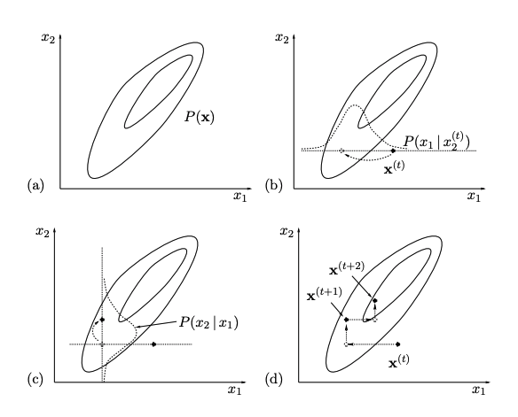
On each iteration, we start from the current state $\mathbf{x}^{(t)}$ and $x_1$ is sampled from conditional density $P(x_1|x_2)$, with $x_2$ fixed to $x_2^{(t)}$. Then $x_2$ is sampled from conditional density $P(x_2|x_1)$, with $x_1$ fixed to $x_1^{(t+1)}$. This gives $\mathbb{x}^{t+1}$ and completes the iteration.

Why does Gibbs Sampling work?

• Gibbs Sampling is a special case of Metropolis-Hastings by giving a special proposal distribution which ensures the acceptance ratio if always $1.0$.

• The Gibbs Sampling proposal distribution is

\[Q(x'_i,\mathbf{x}_{-i}|x_i,\mathbf{x}_{-i}) = P(x'_i|\mathbf{x}_{-i})\]

• Applying Metropolis-Hastings to this proposal, we find that samples are always accepted

\begin{aligned} A(x'_i,\mathbf{x}_{-i}|x_i,\mathbf{x}_{-i}) & = \min(1, \frac{P(x'_i,\mathbf{x}_{-i})Q(x_i,\mathbf{x}_{-i}\|x'_i,\mathbf{x}_{-i})}{P(x_i,\mathbf{x}_{-i})Q(x'_i,\mathbf{x}_{-i}\|x_i,\mathbf{x}_{-i})}) \\ & = \min(1, \frac{P(x'_i,\mathbf{x}_{-i})P(x_i|\mathbf{x}_{-i})}{P(x_i,\mathbf{x}_{-i})P(x'_i|\mathbf{x}_{-i})}) \\ & = \min(1, \frac{P(x'_i\|\mathbf{x}_{-i})P(\mathbf{x}_{-i})P(x_i|\mathbf{x}_{-i})}{P(x_i\|\mathbf{x}_{-i})P(\mathbf{x}_{-i})P(x'_i|\mathbf{x}_{-i})}) \\ & = \min(1,1)\\ & = 1 \end{aligned}

Collapsed Gibbs Sampling

A collapsed Gibbs Sampler marginalizes over one of more variables when sampling from the conditional density. For example, for variables $A$, $B$ and $C$, a simple Gibbs sampler will sample from $P(A|B,C)$, $P(B|A,C)$ and $P(C|A,B)$, respectively. A collapsed Gibbs sampler might marginalize over variable $B$ and sample only from $P(A|C)$ and $P(C|A)$ and not sample for $B$ at all.

Topic Models

Collapsed Gibbs Sampling is a popular inference algorithm for topic models. Topic models are applied primarily to text corpora, which learns the structural relationships between the thematic categories. Typically, we use Latent Dirichlet Allocation to represent the model.

A plate diagram of the generative process of a topic model

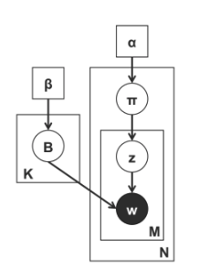
The above plate diagram illustrates a topic model, where we have:

• $\beta$ defines a Dirichlet prior over the topics $B$, where each topic $B_k$ defines a multinomial distribution over the vocabulary.

• $\alpha$ defines a Dirichlet prior over the document.

• $\mathbf{B}$ is the sampled topic.

• $\mathbf{\pi}$ is the document-specific topic distribution or so-called the topic vector.

• $\mathbf{z}$ is the topic assignment.

• $\mathbf{w}$ is the observed word.

When performing the sampling, we first marginalize over the topic $\mathbf{B}$ and the topic vectors $\mathbf{\pi}$ and then sampling from $P(z_i|\mathbf{z}_{-i},\mathbf{w})$, which is a product of two Dirichlet-Multinomial conditional distributions:

\[P(z_i=j\|\mathbf{z}_{-i},\mathbf{w}) \propto \frac{n^{w_i}_{-i,j}+\beta}{n^{(\cdot)_{-i,j}}+W\beta} \frac{n^{(d_i)_{-i,j}}+\alpha}{n^{(d_i)}_{-i,\cdot}+T\alpha}\]

where

• $n^{w_i}_{-i,j}$ is the number of word positions $a$ (excluding $w_i$) such that $w_a=w_i$ and $z_a=j$

• $n^{(\cdot)_{-i,j}}$ is the number of word positions $a$ in the current document $d_i$ (excluding $w_i$) such that $z_a=j$

• $n^{(d_i)_{-i,j}}$ is the number of word positions $a$ (excluding $w_i$) such that $z_a=j$

• $n^{(d_i)}_{-i,\cdot}$ is the number of word positions $a$ in the current document $d_i$ (excluding $w_i$)

We then perform normal Gibbs Sampling on the above distribution to sample $z_i$.

Practical Aspects of MCMC

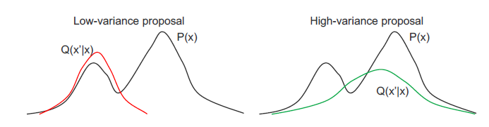
How do we know if our proposal is any good? – Monitor the acceptance rate:

Choosing the proposal $Q(x’ | x)$ is a tradeoff. The ‘narrow’, low-variance proposals have high acceptance, but may take many iterations to explore $P(x)$ fully because the proposed $x$ are too close. The ‘wide’, high-variance proposals have the potential to explore much of $P(x)$, but many proposals are rejected which slows down the sampler.

A good $Q(x’ | x)$ proposes distant samples $x’$ with a sufficiently high acceptance rate.

Acceptance rate is the fraction of samples that MH accepts. A general guideline is proposals should have ~0.5 acceptance rate .

If both $P(x)$ and $Q(x’ | x)$ are Gaussian, the optimal acceptance rate is ~0.45 for D=1 dimension and approaches ~0.23 as D tends to infinity .

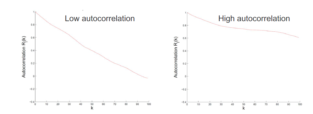
How do we know if our proposal is any good? – Autocorrelation function:

MCMC chains always show autocorrelation (AC), because we are using the previous example to define the transition of the next example. (Note: AC means that adjacent samples in time are highly correlated.) We quantify AC with the autocorrelation fucntion of an r.v.x:

\[R_x(k) = \frac{\sum_{t=1}^{n-k}(x_t-\bar{x})(x_{t+k}-\bar{x})}{\sum_{t=1}^{n-k}(x_t-\bar{x})^2}\]

The first-order AC $R_x(1)$ can be used to estimate the Sample Size Inflation Factor (SSIF):

\[s_x = \frac{1+R_x(1)}{1-R_x(1)}\]

If we took $n$ samples with SSIF $s_x$, then the effective sample size is $n/s_x$. High autocorrelation leads to smaller effective sample size. We wan proposals $Q(x’ | x)$ with low auto correlation.

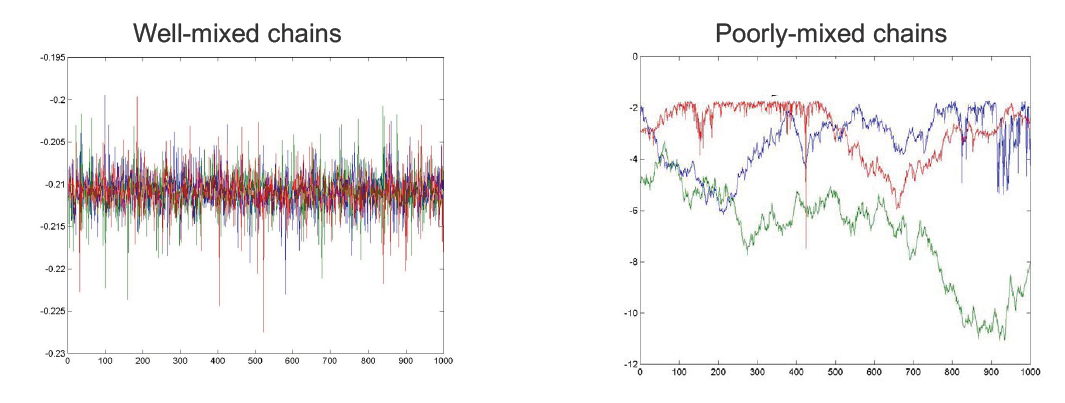
How do we know when to stop burn-in? – Plot the sample values vs time

We can monitor convergence by plotting samples (of r.v.s) from multiple MH runs (chains). (Note: In practice, when people do MCMC, they usually start with multiple MCMC chains rather than one MCMC). If the chains are well-mixed (left), they are probably converged. If the chains are poorly-mixed (right), we should continue burn-in.

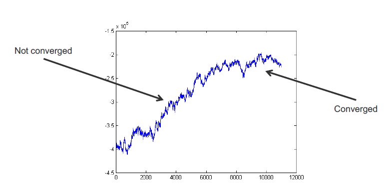
How do we know when to stop burn-in? – Plot the log-likelihood vs time

Many graphical models are high-dimensional, so it is hard to visualize all r.v. chains at once. Instead, we can plot the complete log-likelihood vs. time. The complete log-likelihood is an r.v. that depends on all model r.v.s. Generall, the log-likelihood will climb, then eventually plateau.

Summary

The key point is that we are going to use an adaptive proposal. And we are going to have choices of further engineered adaptive proposal to be a conditional distribution of a single random variable given the rest. And by using the Markov Blanket concept, we can make that simple proposal eqsy to manpulate, and get a constant 1 acceptant rate. So that the samples can be better used. We need to take care of convegence rate, good mixing, etc.

In summary:

• Markov Chain Monte Carlo methods use adaptive proposals $Q(x’ | x)$ to sample from the true distribution $P(x)$.
• Metropolis-Hastings allows you to specify any proposal $Q(x’ | x)$. Though chooing a good $Q(x’ | x)$ requires care.
• Gibbs sampling sets the proposal $Q(x’ | x)$ to the conditional distribution $P(x’ | x)$:
  1. Acceptance rate is always 1!
  2. But remember that high acceptance usually entails slow exploration
  3. In fact, there are better MCMC algorithms for certain models
• Knowing when to halt burn-in is an art.

Optimization in MCMC: Introduction

One of the struggle people had in all vanilla MCMC methods is so called random walk behavior, which is caused by the proposed distribution. However, we want to propose prefered biased samples. How to impose the derivative (maybe likelihood function) into the proposal in a mathematically elegent fashion had became an important question

Hamiltonian Monte Carlo

Hamiltonian Dynamics comes form physics, is given by

\[H(p,x) = U(x) + K(p)\]

Where $x$ is the position vector, $p$ is the momentum vector. $U(x)$ is the potential energy and $K(p)$ stands for kinetic energy. There are many interesting connections betrween the terms and derivatives over Hamiltonian. One of the key of Hamiltonian is that

\[\frac{d x_i}{dt} = \frac{\partial H}{\partial p_i}\] \[\frac{d p_i}{dt} = - \frac{\partial H}{\partial x_i}\]

When we want to sample a target distribution, we can leverage on gradient methods by introducing more variables to an auxiliary distribution.

\(P_H (x,p) = \frac{e^{-E(x)-K(p)}}{Z_h}\) Thus, using Hamiltonian, we are able to define the change of state v.s. the gradient of a loss function over the change.

How to update: Euler’s Method

There are multiple way to compute the $\delta$ in the state as a function of teh gradient. The Euler’s Method directly estabilsh the change in $p$ (momentum), and $q$ (position) as a function of the loss.

\[p_i(t + \epsilon) = p_i(t) + \epsilon \frac{dp_i}{dt}(t) = p_i(t) - \epsilon \frac{\partial U}{\partial q_i}(q(t))\] \[q_i(t + \epsilon) = q_i(t) + \epsilon \frac{dq_i}{dt}(t) = q_i(t) + \epsilon \frac{ p_i(t) }{m_i }\]

How to update: Leapfrog Method

Leapfrog Method is prefered, because it alternates between the $p$ and $q$ to calculate the updates in a very controlled fashion. So behaviors like over shooting and under shooting can be avoided. \(p_i(t + \epsilon /2) = p_i(t) - (\epsilon /2) \frac{\partial U}{\partial q_i}(q(t))\)

\[q_i(t + \epsilon) = q_i(t) + \epsilon \frac{p_i(t + \epsilon /2)}{m_i}\] \[p_i(t + \epsilon) = p_i(t + \epsilon /2) - (\epsilon / 2) \frac{\partial U}{\partial q_i}(q(t + \epsilon))\]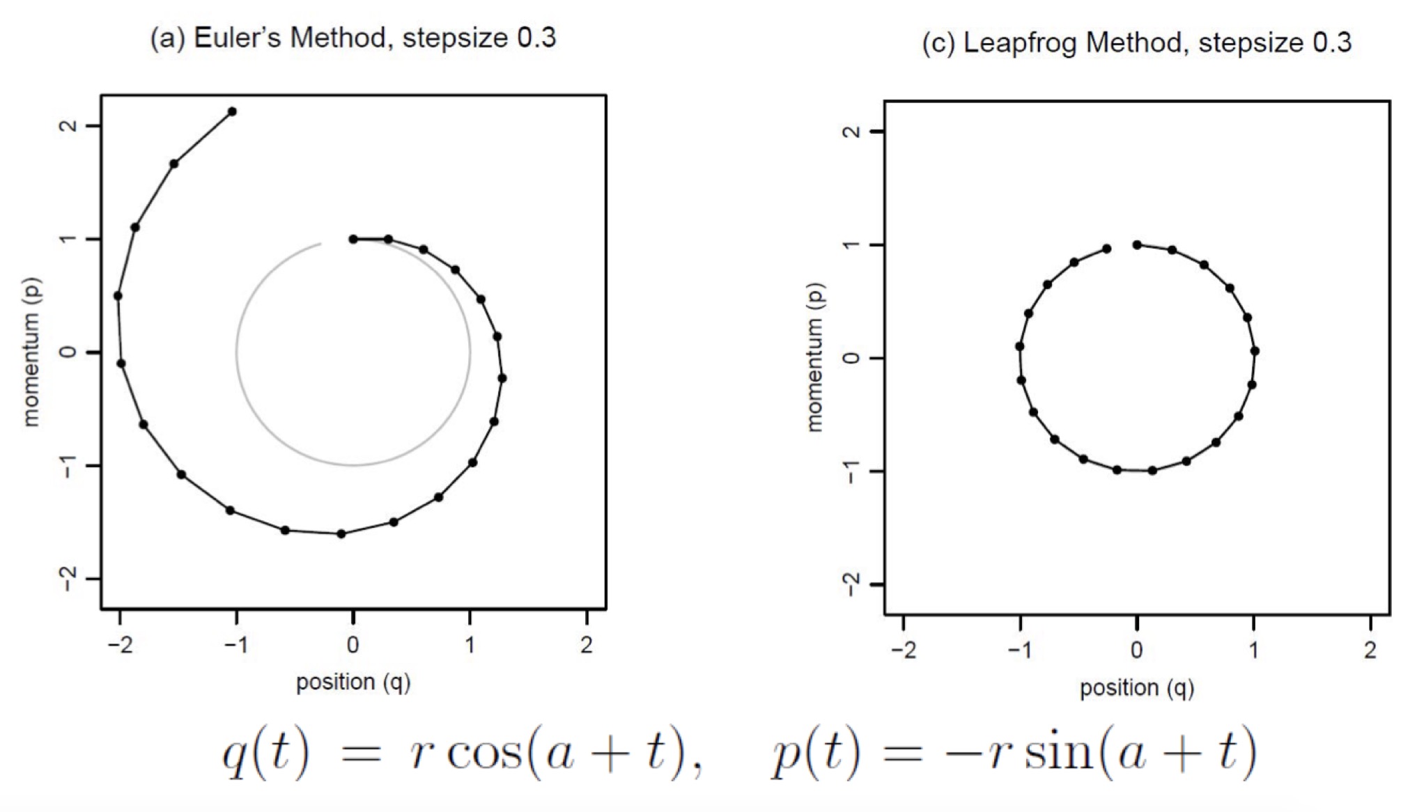

MCMC from Hamiltonian Dynamics

Let $q$ be variable of interest, $p$ is introduced as an auxiliary random variable in order to define the Hamiltonian.

\[P(q,p)=\frac{1}{Z} \exp (-U(q)/T) \exp(-K(p)/TY)\]

Where $U(q) = -log [\pi (q) L(q|D)]$ and $K(p) = \sum^d_{i=1} \frac{p^2_i}{2m_i}$. Here it is a Bayesian setting where we have both the distribution of hidden states or the states of interest and also conditioned from priors. $U(q) = -log [\pi (q) L(q|D)]$ connects to the likelihhod, the gradient of which is not directly involved in the proposal of next $q$. Then a accept/ reject critera is built based on the change of the Hamiltonian.

Langevin Dynamics

Langevin Dynamics is special case of Hamiltonian. Instead of doing Leapfrog, Langevin does a more sophiscated update based on second-order updates of the sampling states.

\[q^*_i = q_i - \frac{\epsilon^2}{2} \frac{\partial U}{ \partial q_i}(q) + \epsilon p_i\]

\(p^*_i = p_i - \frac{\epsilon}{2} \frac{\partial U}{ \partial q_i}(q) - \frac{\epsilon}{2} \frac{\partial U}{ \partial q_i}(q^*)\) Even for a strange distribution with constrains on regions, this augmented optimization methods still deal with it.

Optimization in MCMC: Conclusion

• Using Hamiltonian, we are able to define the change of state v.s. the gradient of a loss function over the change.
• Hamiltonian Mento Carlo can improve acceptence rate and give better mixing by incorporating optimization based approaches to generate better proposals.
• Stochastic variants can be used to improve performance in large dataset scenarios.
• Hamiltonnian Mento Carlo may not be used for discrete variable