Lecture 15: Statistical and Algorithmic Foundations of Deep Learning

How graphical models relate to deep learning.

Neural Network Review

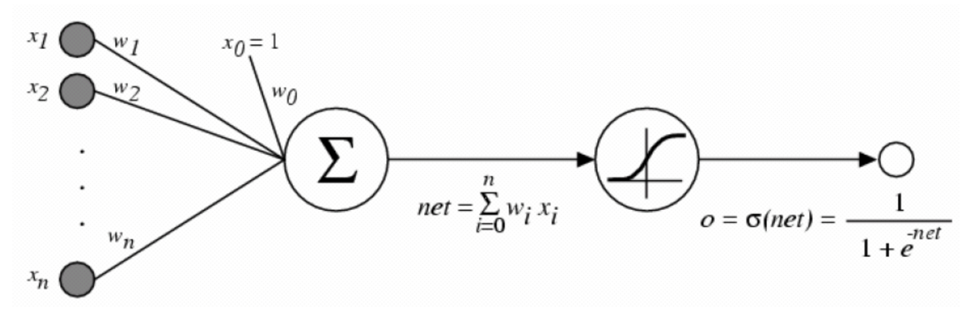
The Perceptron/Perceptron Learning Algorithm

The most simple neural network is the perceptron. It applies a weighted sum to its inputs, and applies a sigmoid function to this sum (shown as the $ \sigma $ below).

This learning algorithm can be used to maximize a conditional likelihood, $y=f(x)+\epsilon$, such that

\[\bar{w} = \arg \min_{\bar{w}} \sum_i \frac{1}{2} (y_i - \hat{f} (x_i ; w))^2\]

Thus, we can find the gradient of this loss function with respect to a weight $w_j$:

\[\begin{aligned} \frac {\partial E_D [\bar{w}]}{\partial w_j} &= \frac {\partial}{\partial w_j} \frac{1}{2} \sum_d (t_d - o_d)^2 \\ &= \frac{1}{2} \sum_d 2 (t_d - o_d) \frac {\partial}{\partial w_j} (t_d - o_d) \\ &= \sum_d (t_d - o_d) \frac {- \partial o_d }{\partial w_j} \\ &= - \sum_d (t_d - o_d) \frac { \partial o_d }{\partial net_d} \frac { \partial net_d }{\partial w_i} \\ &= - \sum_d (t_d - o_d) o_d (1-o_d) x_d^i \\ \end{aligned}\]

So, $\nabla E_d [\bar{w}] = - (t_d - o_d) o_d (1-o_d) \bar{x_d}$. Thus, the incremental perception learning algorithm does the following (with a learning rate of $\eta$):

For each training example $d$ in $D$:

1. compute gradient $\nabla E_d [\bar{w}]$
2. $\bar{w} = \bar{w} - \eta \nabla E_d [\bar{w}]$

This can also be done in batch mode, by averaging gradients across multiple examples.

Backpropagation using a computational graph

This learning algorithm gets slightly more complicated when we introduce hidden units, circled in yellow below:

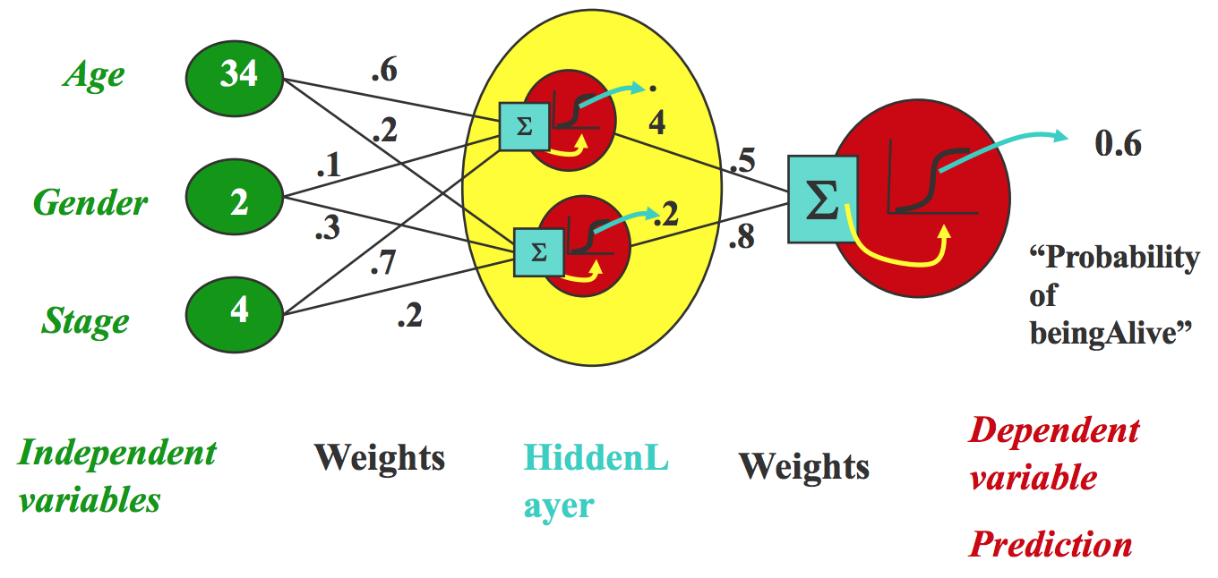
Unlike neurons in the final layer, hidden units do not correspond to a particular class. We train the weights in these layers using backpropagation, or “reverse-mode differentiation”. First, we can build a computaitonal graph, where $x$ is the input and $f(x)$ is the output, and nodes 2, 3, and 4 are the intermediate computations:

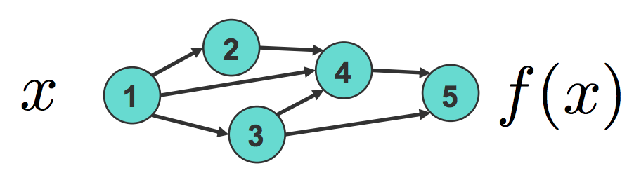
By applying the chain rule, we can derive:

\[\frac {\partial f_n}{\partial x} = \sum_{i_1\in \pi(n)} \frac {\partial f_n}{\partial f_{i_1}} \frac {\partial f_{i_1}}{\partial x} = \sum_{i_1\in \pi(n)} \frac {\partial f_n}{\partial f_{i_1}} \sum_{i_2\in \pi(i_1)} \frac {\partial f_{i_1}}{\partial f_{i_2}} \frac {\partial f_{i_2}}{\partial x} = \cdots\]

This algorithm of recursively calling the chain rule is called backpropagation, and we can use it to train most deep networks, even though we don’t have a target for the hidden units.

Modern building blocks of deep networks

Most deep networks are composed of many simple building blocks:

1. Layers, specifying the architecture and type of connections
   • Fully connected
   • Convolutional and pooling
   • Recurrent
   • Residual Layers
   • etc.
2. Activation functions, that go in between these layers
   • Linear: $f(x) = x$
   • ReLU: $f(x) = max(0, x)$
   • Sigmoid: $f(x) = \sigma(x) = \dfrac{1}{1+e^{-x}}$
   • tanH: $f(x) = \text{tanh}(x) = \dfrac{e^x - e^{-x}}{e^{x} + e^{-x}}$
   • etc.
3. Loss functions, which we are trying to minimize (can have many in one network)
   • Cross-entropy loss
   • Mean squared error
   • etc.

Feature learning

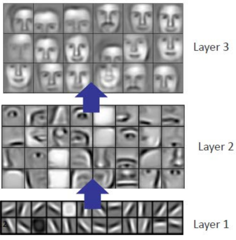
Often one important goal of deep networks is to learn a good representation of the input. Deep networks are often good at doing this, and can attempt to get a “disentangled” representation, i.e. amenable to linear separation, as shown below:

Because DNNs have this property, it is often possible to transfer representations and use pretrained deep neural networks as feature extractors for new tasks. In these cases, the activations of intermediate layer $h_j$ in model $M$ (trained on task $A$) are used to generate representations for a different task $B$. Because these representations might be linearly separable, it typically suffices to train a linear model, or shallow neural network on the featurized data. The most common example of this is ImageNet, and models trained on ImageNet (i.e. vgg16) are typically good feature extractors for other vision based tasks.

Graphical Models vs. Deep Networks

While the two paradigms appear to share the same graphical structure on the surface, juxtaposing their properties point out subtle differences between them.

Feature	Graphical model	Neural Networks
Representation	It encodes prior meaningful knowledge. Every node has a meaning and edges represent the relationship between the variables.	They are learnt in a way that optimizes the end metric. The meaning of intermediate nodes are typically not the focus.
Learning and inference	Involves well studied algorithms like MCMC, VI and message passing.	Learning primarily involves gradient descent. Inference just involves a forward pass through the network.
Structural utility	Graphs help monitor theoretical and empirical behaviour of inference	Networks facilitate the organization of computational operations

Tradeoffs: As with any modeling strategy, there are inherent tradeoffs between graphical models and neural networks. Graphical models allow us to directly encode prior knowledge about the world into the structure of the model (i.e. latent states), enabling us to enforce some weak notions of causality. However, this requires domain expertise, and assumes that the structure enforced on the model is the most natural/well suited for the task. In contrast, neural networks learn their own latent representations, by minimizing loss in an end-to-end manner. As a result, they may be seen as learning a more ‘efficient’ representation. However, this approach can require signicant amounts of data, which may not always be available.

Thus, we see that the graphs in a graphical model represent the model itself whereas it just represents computation in the case of a deep network.

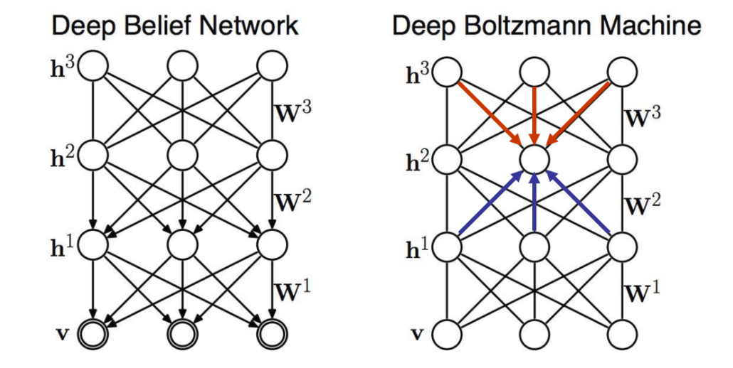
Some neural networks can be completely understood as a conventional graphical model. A few examples are examined below -

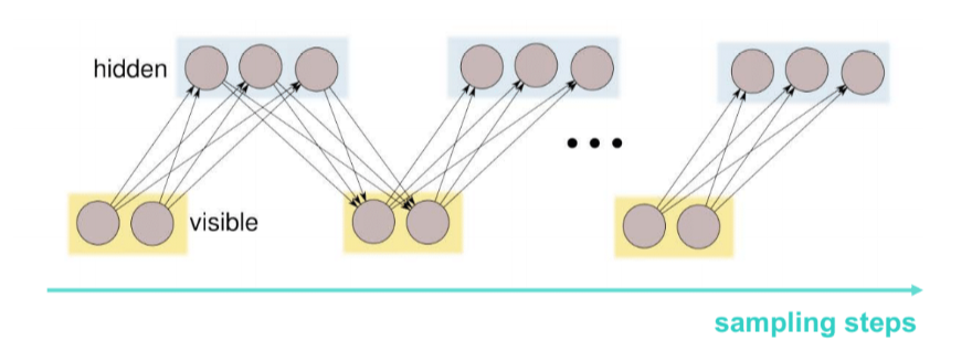
1.Restricted Boltzmann Machines

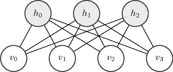
Overview: RBMs are represented by undirected bipartite graphs, with one “visible” layer and a second “hidden” layer. There are no connections between nodes in the same layer (in contrast to unrestricted Boltzmann machines, which permit connections between hidden units).

Learning: We compute a loss function by marginalizing over all the hidden variables and taking the derivative w.r.t weights:

\[\log L(v) = \log \sum_{h} \exp(\sum_{i,j} w_{ij} v_{i} h_{j} + \sum_{i} b_{i}v_{i} + \sum_{j} c_{j} h_{j} - \log(Z))\] \[\frac{\partial \log L(v)}{\partial w_{ij}} = \sum_{h} P(h | v) \frac{\partial}{\partial w_{ij}} P(v,h) - \sum_{v,h} P(v,h) \frac{\partial}{\partial w_{ij}} P(v,h)\]

or alternatively, as: \(\dfrac{\partial}{\partial w_{ij}} \log L(v) = \mathbb{E}_{P(h|v)} \bigg[\dfrac{\partial}{\partial w_{ij}} P(v, h)\bigg] - \mathbb{E}_{P(v, h)} \bigg[\dfrac{\partial}{\partial w_{ij}} P(v, h)\bigg]\)

Of the two terms in the loss above:

• The first term is the expectation taking over the conditional of the hidden given the observed, i.e. we average over the posterior. This is computed via sampling, which is exact (the RBM factorizes over $h$ given $v$). In neural network literature, this is also called the clamped/ wake/ positive phase.
• The second term is the expectation taken over all random variables (both hidden and observed), i.e we average over the joint. This is also computed sampling, but requires the iterative Gibbs sampling algorithm. Consequently, it’s far more expensive (computationally) and slow to converge. In neural network literature, this is called the the unclamped/ sleep/ negative phase.

2. Sigmoid Belief Networks

SBNs consist of stacks of directed linear layers combined via non-linear sigmoid activation functions. The intermediate meaning of the hidden layers are typically ignored and so even though they synactically represent graphical models, operationally they begin to deviate. Operationally treating them as graphical models, leads to inefficient inference because of the implicit “explaining away” phenomenon as when we want to infer a hidden variable, it is coupled with all other hidden random variables in that layer. This stands in contrast to the RBM case because d-seperation in the RBM graph meant that the hidden random variables are independent given the other layer. Also, unlike the RBM, computing the conditional does not involve a negative phase.

We now connect our discussions of inference in the SBN and the RBM. Recall that for the gradient of the sleep phase of loss function, we could sample the joint using Gibbs procedure which alternates between different subsets of varaibles. While the vanilla Gibbs sample requires sampling every single random variable one by one given all other points, a broader idea, called block Gibbs sampling which groups the variables into arbitrary blocks and samples on the block given everything else. In the case of the RBM, we consider the two layers as two blocks and hence, sampling involves alternating between the two layers.

Note here that the conditional distributions $P(v \| h)$ and $P(h \| v)$ are represented by sigmoids. Thus, Gibbs sampling of the joint of an RBM can be viewed as a top down pass in an infinitely deep SBN with tied weights. ## 3. Deep Belief Networks Independently of SBNs, people approached the problem of training deep architectures from a different lens and arrived at Deep Belief Nets. As discussed earlier, approaching the problem using exact inference is problematic due to the "explaining away" effect. Instead, Deep Belief Nets approach the problem as hybrid graphical models which learn to extract deep hierarchical representations of the training data by stacking RBMs trained in a greedy manner followed by some ad-hoc fine-tuning. More concretely, DBNs represent a joint probability distribution $$ P(v,h^1,h^2,h^3) = P(h^2,h^3) P(h^1|h^2) P(v|h^1) $$ where v are the visible variables and $ h^1 $, $ h^2 $ and $ h^3 $ are the hidden variables as shown in the figure below. Here, $ P(h^2,h^3) $ is an RBM and the conditionals $ P(h^1 \vert h^2) $ and $ P(v \vert h^1) $ are represented as sigmoid activations over a linear layer. As described earlier, directly performing inference and maximizing the likelihood of the joint is problematic. Hence we resort to a greedy layer-wise pretraining strategy described below:

### Layer-wise pre-training The principle of greedy layer-wise unsupervised pre-training can be described as follows: - **Pre-train and freeze the first RBM** : Train the first layer as a standard RBM with the data being fed in at the visible layers. - **Obtain the hidden layer samples $ p(h^1 \vert h^0) $** : Use the trained RBM to get corresponding hidden samples for each data point by computing $p(h^1 \vert h^0)$ for each point in the training set. - **Train another RBM using samples obtained** : Use the hidden layer samples obtained in the previous step to train another RBM where these samples are fed in at its visible layers. Note that, the first RBM remains fixed during this step. - **Iterate the previous two steps** : Repeat the procedure in previous two steps to train the desired number of layers by training successive RBMs using the hidden samples from the previous layer. Note that at any point, the last RBM (say the $N^{th}$ RBM) trained can be unrolled infinitely to produce an infinite belief network with the first N-1 layers given by the weights of the first N-1 trained RBMs and all the layers after that being represented using tied weights given by the $N^{th}$ RBM. Hence, each additional RBM trained can be viewed as untying an additional layer and freezing that layer of weights while fine-tuning all the following layers of the infinite belief network. Eg. In the figure below, the first 2 layers have been frozen and untied from the training procedure while all the layers starting from W3 are being trained as a standard RBM. After pre-training the N RBMs, we simply stack them in the order in which they were trained to obtain an initialization of the DBN.

### Fine-tuning Since the procedure followed above is pretty ad-hoc, it is unlikely to lead to a good probabilistic/generative model. However, the representations learnt can be useful for other downstream task. Some examples of possible use cases for these representations could be : - **Unsupervised Learning (DBN -> Autoencoder)**: Autoencoders are a useful model class for compressing the input data to a low dimensional representation from which input can be decoded back without much loss of information. DBNs by themselves might not be able to find an ideal compression but the weights trained using the pre-training procedure might be able to provide a good initialization for the model. The procedure for fine-tuning a DBN to obtain an Autoencoder can be described as follows: - Pre-train a stack of RBMs in a greedy layer-wise fashion as described in the previous section with successively fewer hidden units in each successive RBM as shown in the figure below. - Unroll the RBMs to create an autoencoder as shown in the figure below. - Fine-tune the parameters by backpropagating the reconstruction error and optimizing using gradient descent. - **Supervised Learning (DBN -> classifier)**: The representations learnt by the DBN might not be very useful for classifying the data, but it can serve as a good initialization to further fine-tune the network to obtain useful representations. The procedure in this case can be described as follows: - Pre-train a stack of RBMs in a greedy layer-wise fashion as in the autoencoder case. - Unroll the RBMs to create a feed-forward classifier. - Fine-tune the parameters by backpropagating the classification error and optimizing by gradient descent.

## DBM: Deep Boltzmann Machines

DBMs are a fully undirected extension of DBNs. They can be trained using a similar procedure as RBMs using MCMC or using a variational approximation of the data distribution and subsequently doing greedy layerwise pre-training as in the case of DBNs. As with DBNs these can also be used to initialize other networks for downstream tasks. ## RBM v.s. optimization steps We have so far looked at the optimization in RBMs/infinite belief nets as an inference procedure to progressively infer the values of the hidden states given the observed/visible states. Now imagine that the input/observed variables given to the RBM are actually the initial parameters of another model. In this case each unrolled RBM layer can be seen as an update or optimization step on the parameters of the other model. This [meta-learning](https://en.wikipedia.org/wiki/Meta_learning_(computer_science)) setup has been proposed recently in using RNNs to unroll the optimization steps. proposed a method to find the optimal steps to take given a fixed number of optimization steps. This can be represented as: $$ y^*(x,w) = \text{opt-alg}_y E(y,x;w) $$ Here, $y^*$ is a non-linear differentiable function of the inputs and weights. Hence, we can impose some loss and optimize it as any other standard computation graph using backprop. Similarly, message passing based inference algorithms which can be truncated and converted into computational graphs and subsuquently optimizing the objective containing the approximate marginals (computed using the truncated message passing) directly to obtain better message passing and faster convergence. ## Concluding remarks on Graphical Models vs. Deep Networks - Classical graphical models are concerned with the correctness of learning and inference of all variables - Deep networks are more concerned about representing the observed variables using the hidden variables. Hence the focus here is somewhat different: - The primary goal of deep generative models is to represent the distribution of the observable variables. Adding layers of hidden variables allows to represent increasingly more complex distributions. - Hidden variables are secondary (auxiliary) elements used to facilitate learning of complex dependencies between the observables. - Training of the model is ad-hoc, but what matters is the quality of learned hidden representations. - Representations are sometimes judged by their usefulness on a downstream task (the probabilistic meaning of the model is often discarded at the end). Hence, concepts of generalization and transferability sometimes become more important than exact inference or correctness. ## Supplementary **Combining Sequential NNs and GMMS** : Inference is performed via a forward-backward algorithm, while weights are learned use standard SGD by backpropogation.