Lecture 16: Building Blocks of Deep Learning
Overview of CNNs, RNNs, and attention.
Convolutional Neural Networks (CNNs)
CNNs are biologically-inspired variants of MLPs that exploit the strong spatial local correlations present in images. The biological concept of the receptive field states that the visual cortex contains a complex arrangement of cells that are sensitive to small sub-regions that are tiled to cover the visual field. CNNs enjoy sparse connectivity, shared weights, and a hierarchy of representation. Stacking multiple layers can result in lower layers learning low-level features, while upper layers learn high-level representations. Using the biological analogue, simple cells detect local features while complex ones pool the outputs of simpler cells.
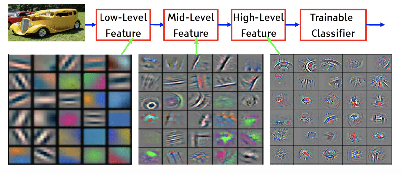
One type of layer in a CNN is the convolutional layer. These involve taking taking filter kernels and convolving them over the image. This has the effect of filtering an image and preserves the local connectivity of an image. The use of convolutions also allows for parameter sharing, whereby the same parameters (i.e., each filter kernel) can be applied to multiple parts of the same image to greatly reduce the model’s complexity. This process creates a feature map from the responses for each filter, which can be fed into a pooling layer. The pooling layer helps to reduce the dimensionality of the input space by downsampling the feature maps at each layer. For example, max pooling with a kernel size of 2x2 only takes the max pixel response in each set of 2x2 pixels. This downsamples the image by a factor of 4. Average pooling would instead take the average of the pixels in a kernel. The advantage of pooling is to improve robustness to the exact spatial location of features, as anything that is “close enough” would be pooled into the same output. Many CNNs involve stacking multiple alternating convolution and pooling layers together to build the aforementioned hierarchy of representation.
Examples of ConvNets show a trend towards ever increasing numbers of layers:
- AlexNet, 8 layers
- VGG, 19 layers
- GoogLeNet, 22 layers
- ResNet, 152 layers
Recurrent Neural Networks (RNNs)
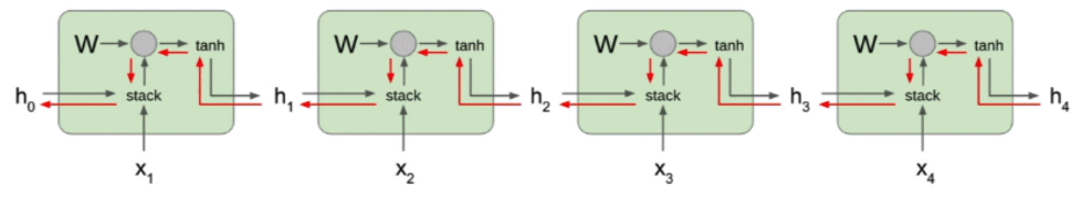
The temporal (or sequential) analogue to the CNN is the RNN. RNNs can have a variable number of computation steps unlike CNNs. Unlike MLPs and CNNs, RNN outputs depend not only on the current input, but also on the previous states of hidden layers.
LSTMs and the Vanishing/Exploding Gradient Problem
Unrolling an RNN for several steps results in multiple products with W and applying tanh multiple times. The hidden states that are passed on to each successive cell follow this expression:
\[h_t = tanh(W^{hh} h_{t-1} + W^{hx} x_t)\]As you backpropagate backward to $h_0$, there will be many repeated factors of W and tanh.
If the singular value of the W matrix is greater than 1, this can result in exploding gradients; similarly, singular values under 1 can result in vanishing gradients.
This is because product over the W matrices during backprop will result in either exponential growth/decay in value.
A solution to this problem is to use gradient clipping
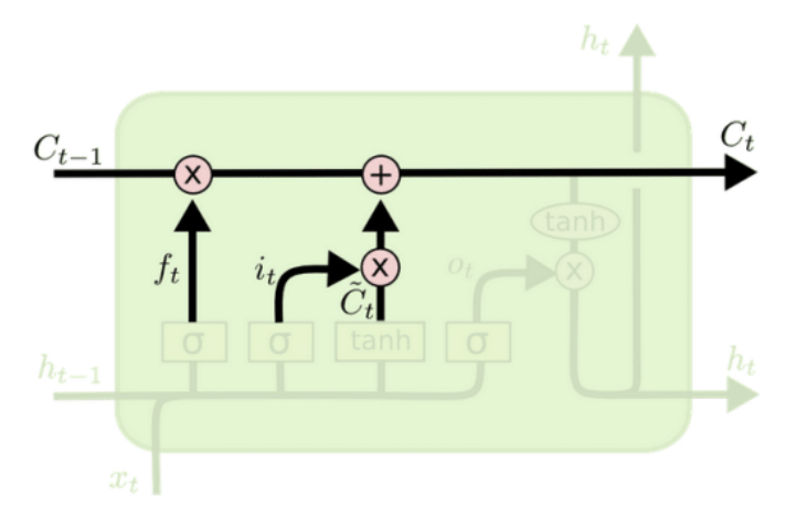
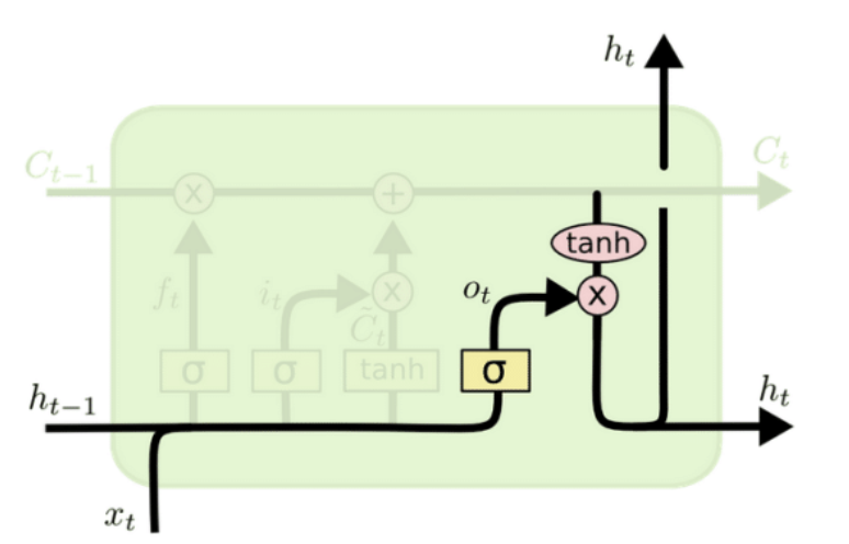
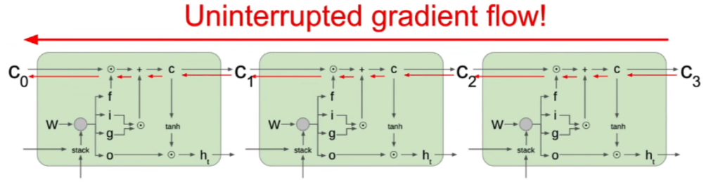
LSTMs are designed to solve the long-term dependency problem by creating a path with uninterrupted gradient flow during backpropagation
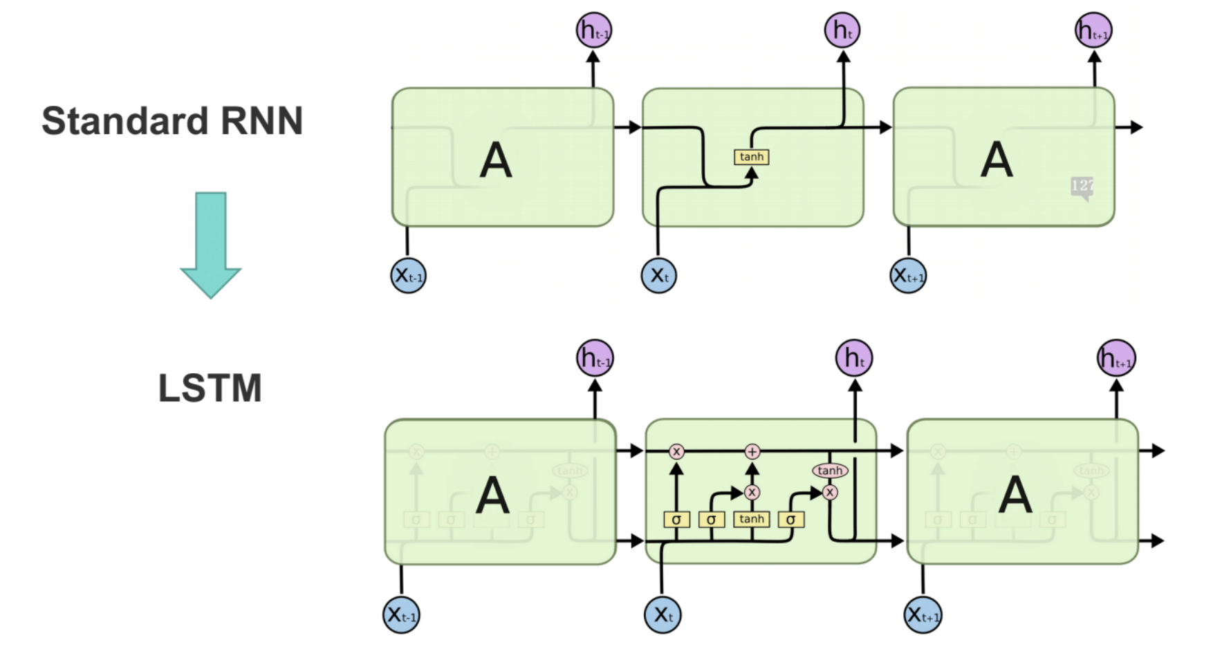
They use linear memory cells and multiplicative gates to store read, write, and reset information.
- Forget gate: decides what must be removed from $h_{t-1}$.
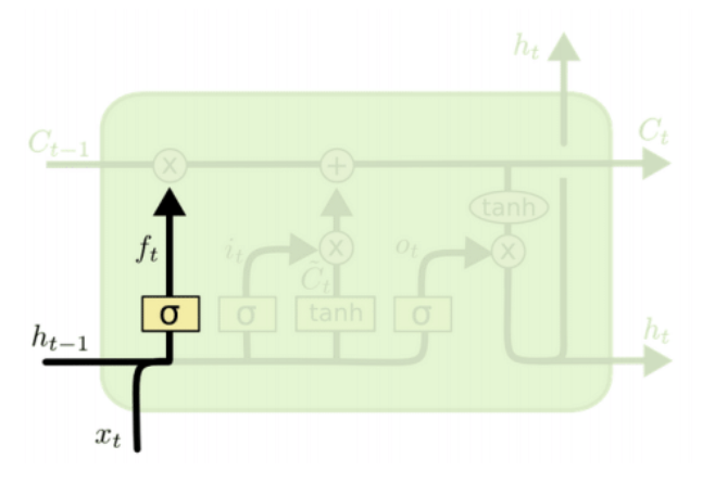
- Input gate: whether to write to cell and what information should be stored
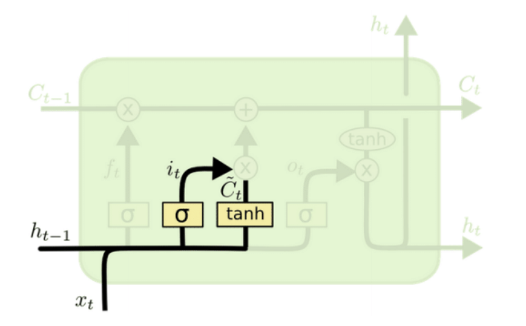
- Update cell state: $f_t$ controls how much of $C_{t-1}$ is forgotten. $i_t$ scales our new candidate values by how much we want to update each state value.
- Output gate: decides what to output from the cell state
The sigmoid in $o_t$ decides which part of the cell state will be outputted.
As can be seen, LSTMs allow for a path with uninterrupted gradient flow, which helps mitigate the long-term dependency problem. There is no need to multiply by the W matrix during backprop, which was the source of the growth/decay; instead, you multiply by the different values of the gates. While this does not totally eliminate the vanishing/exploding gradient problem, it makes it much less likely, as there is usually a path where the gradient does not explode/vanish.
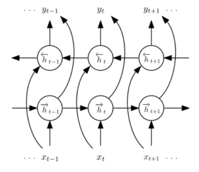
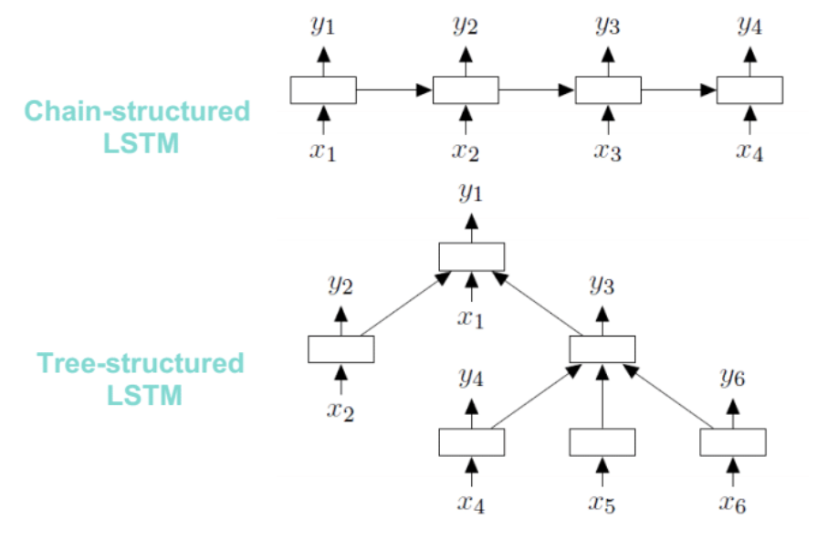
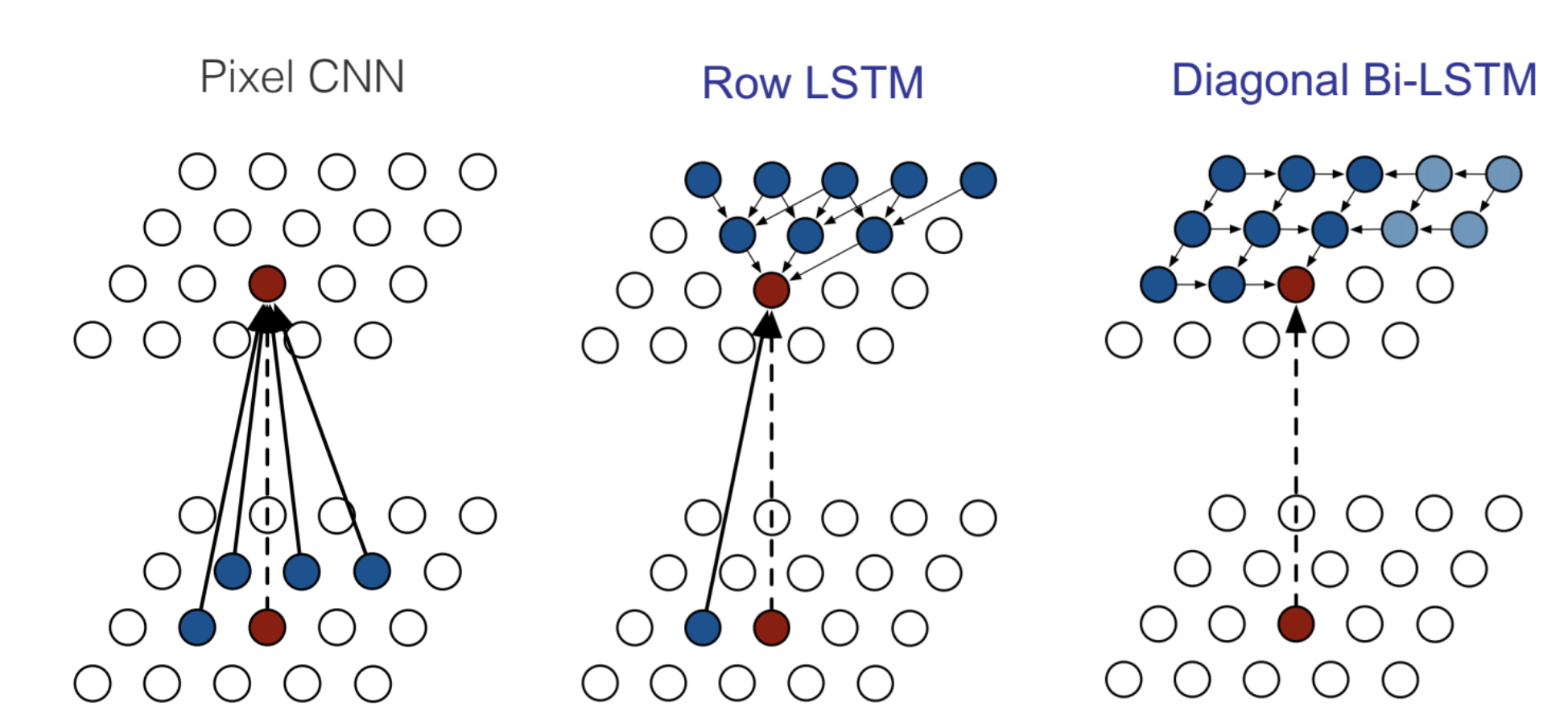
Different Flavors of RNNs
- Bi-directional RNN: The hidden state is the concatenated result of both forward and backward hidden states so that it can capture past and future information.
- Tree-structured RNN: Allows for the hidden states to be conditioned on an input and the hidden states of arbitrarily many child units. The standard LSTM, for example, is a special case conditioned on only one child unit.
- RNNs for 2D Sequences: Fixed structures for 2D images that capture different dependencies and hierarchical relations.
- RNNs for Graph Structures: Used in image segmentation.
Attention Mechanisms
Attention mechanisms are techniques that are used to focus on particular features in the data. They has been show to drastically improve performance in tasks such as machine translation, image captioning and speech recognition. They allow to accomodate for long-range dependencies, and dealing with the problem of vanishing gradients, seen in RNNs. By allowing for fine-grained localized representations of portions of data, like patches in images or words in sentences, attention improves feature recognition in the model.
Attention Computation
Attention can be computed for a machine translation task using the following procedure:
- Encode each token in the input sentence into a key vector.
- When decoding, compare the query vector with the encoder states, and generate alignment scores corresponding to each key vector.
- Compute the attention weights by normalizing the alignment scores.
- Treat the encoder states as value vectors and compute a weighted sum, using the attention weights.
- Use this weighted sum in the decoder to generate the next token.
Attention Variants
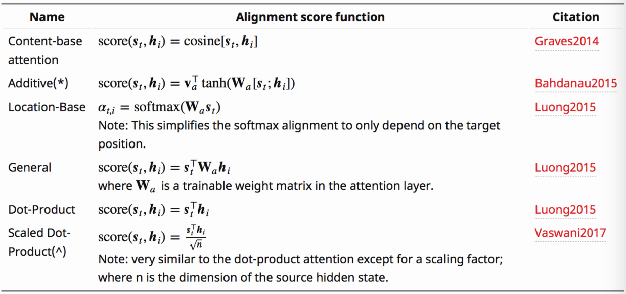
There are a number of different alignment score functions that may be used to generate scores. Some of these are shown in the table below:
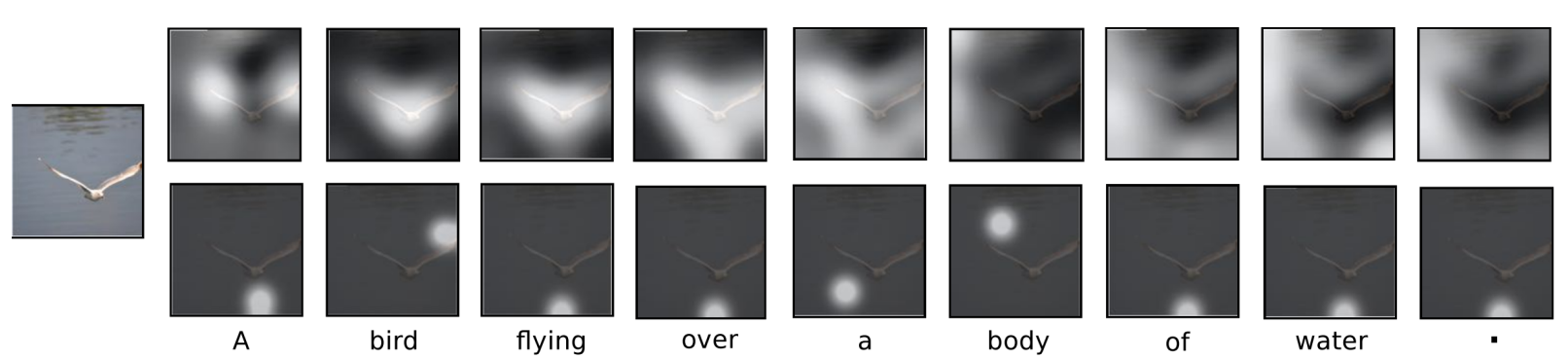
Soft and hard attention are variants of attention that respectively use deterministic and stochastic methods in computing the weights for each token. The computation described above is for soft attention. Instead of using the attention weights to compute a weighted average, hard attention uses these as probabilities and samples from the corresponding features using this distribution. A comparison for attention used on images can be illustrated below. Notice how soft attention can be diffuse, and assign nonzero weights to significant weights to large portions of the image at times, while hard attention focuses on a particular equally-sized part of the image in each case. Soft attention is presently the more popular variant, primarily because it allows for simpler backpropagation in the network.
Applications in Computer Vision
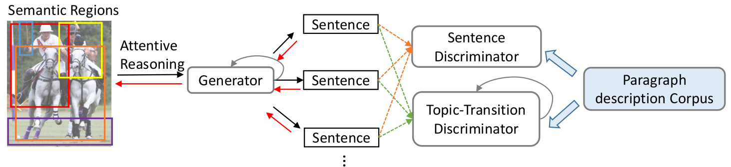
Attention can be used in conjunction with conventional CNNs in image processing. Features extracted from the CNN are used as key vectors and attention is used to sequentialy compute the caption as tokens. It can also be used in image paragraph generation, which is the generation of a long paragraph to describe an image. This is a challenging task because it involves long-term reasoning about language and visual features. Each sentence needs to be grounded on visual features to ensure contentful descriptions. One technique for doing this, presented in Xu et al. (2017)
- The image is first segmented into semantic regions, and each region is locally captioned with phrases
- Attention is applied on the visual regions and the text phrases and the resulting features fed to a generator which generates sentences
- These sentences are then fed to a sentence discriminator and a recurrent topic-transition discriminator for assessing sentence plausibility and topic coherence respectively
- A paragraph description corpus is adopted to provide linguistic knowledge about paragraphgeneration, which depicts the true data distribution of the discriminators
The entire pipeline can be seen in the figure below:
Transformers: Multi-Headed Attention
Transformer
Recently, Vaswani et al. (2017)
As shown below, the Transformer employs multi-headed self-attention, in which multiple attention layers run in parallel. Intuitively, this can enable different heads to focus on different parts of the sequence.
Formally, multiple heads of Queries \(Q\), Keys \(K\) of dimension \(d_k\), and Values \(V\) can be packed together into separate matrices to allow for attention to be computed efficiently using the scaled dot-product variant, which they suggest prevents diminished gradients during training:
\[\text{Attention}(Q, K, V) = \text{softmax}(\frac{QK^\top}{\sqrt{d_k}}) V\]Multi-headed attention can then jointly attend to information from multiple different representations at different positions by:
\[\begin{aligned} \text{MultiHead}(Q, K, V) &= \text{Concat}(\text{head}_1, \ldots, \text{head}_h) W^O \\ \text{where head}_i &= \text{Attention}(QW_i^Q, KW_i^K, VW_i^V) \end{aligned}\]Vaswani et al. (2017) obtain a single-model state-of-the-art BLEU score of 41.8 after training for 3.5 days on eight GPUs, which is two orders of magnitude less training time than recurrent approaches. They visualize the weights of the multiple attention heads to try to explain that each head learns separate information, such as long-term dependencies. Also, they demonstrate the Transformer’s ability to learn structured outputs for English constituency parsing by beating all other discriminative recurrent sequence-to-sequence methods.
BERT: Pre-training of Deep Bidirectional Transformers for Language Understanding
Unsupervised Language Model Pre-training
Recently, language representation via unsupervised language model pre-training has revolutionized the field of natural language processing.
Parameters learned during the training of large language models using self-supervision have been shown to be extremely effective when transferred to other NLP prediction tasks.
ELMo
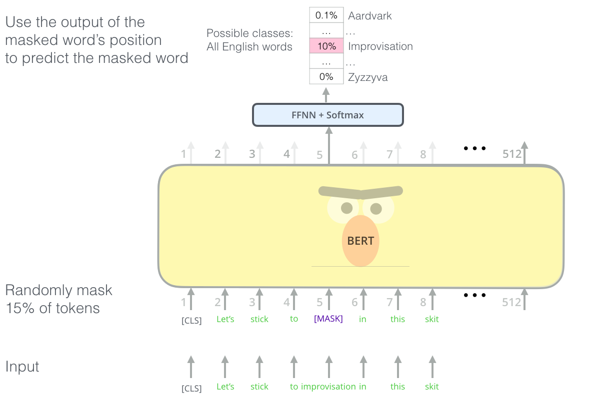
BERT
In BERT (Bidirectional Encoder Representations from Transformers), Devlin et al. (2018)
In the paper, the authors report using both Wikipedia data (2.5B words) and eBook data (800M words) for training a Transformer encoder with hundreds of millions of parameters. An ablation study on model size empirically shows that extreme model sizes lead to large improvements on even very small scale tasks, provided that the model has been sufficiently pre-trained. Although training takes many more steps to converge than a traditional language model objective, BERT, with only single output layer modifications, performs at the state-of-the-art for eleven NLP tasks including sentiment, question answering, and natural language inference. While Google is able to train BERT in just 4 days on 4 TPU pods, training is impractical for academics with traditional GPU resources, For example, a standard 4 GPU desktop with an RTX 2080Ti would take almost 99 days to complete training!