Lecture 17: Deep generative models (part 1)

Overview of the theoretical basis and connections of deep generative models.

In this lecture, we will bring an overview of the theoretical basis and connections between several popular generative models.

Theoretical Basis of deep generative models

Deep Generative Models

GANs and VAE models are heard by many as well as considered by some as one of the most exciting development in machine learning or at least in deep learning over the past decade, and you will see a reason today. But in terms of mathematics, they are not so complicated.

There are deep connections between almost every piece of deep learning and their counterpart machine learning method invented decades ago. For example, deep neural network corresponds to infinite deep computing graph of a one-layer RBM, and infinitely wide deep neural network is actually a finite width Gaussian process.

Deep generative models

• Define probabilistic distributions over a set of variables;
• Deep means multiple layers of hidden variables. (So it is a graphical model.)

Early forms of deep generative models

To ground to a few concrete example, we introduce some early forms of deep generative models.

• Hierarchical Bayesian models

  • Sigmoid brief nets We have learned already sigmoid belief network where the lower layer is conditioning on the previous layer using a conditional distribution defined by a sigmoid function. The lower layer follows a Bernoulli distribution whose parameters are dependent and defined by the sigmoid function. See details below.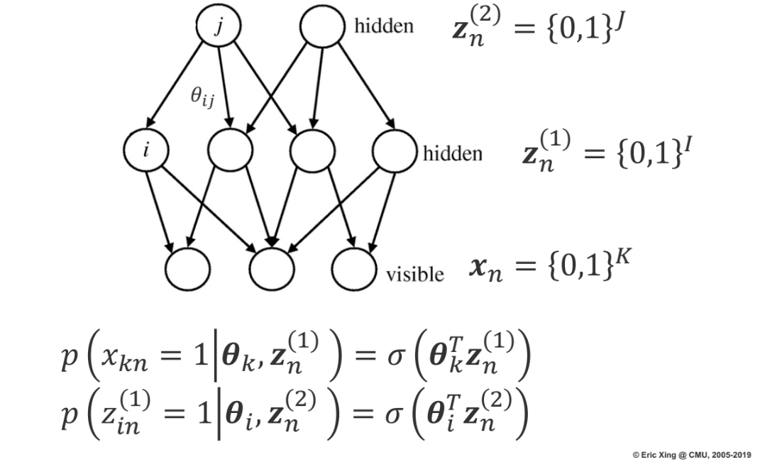

    

    Sigmoid brief nets

    Deep belief network is one of the first deep learning models in its current sense. Train block-wise RBMs and stack them on top of each other and then retrain them using auto-regressive functions or some other heuristics.

    Graphical models have mathematical properties to tell you the behavior, and then the deep learning model/technique is a heuristic extension of that. (The very word ?model? itself is not very proper sometimes because sometimes it is only a technique built on a principled model.)

• Neural network models

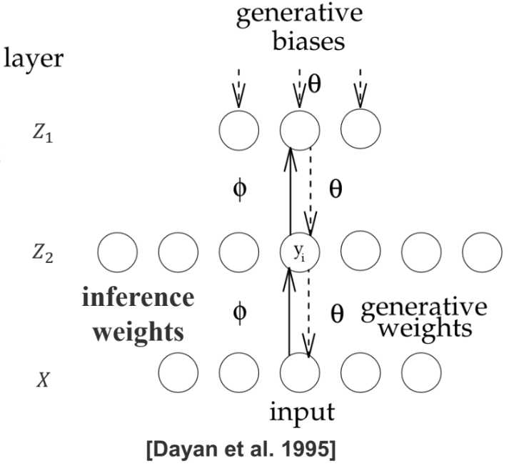
  • Helmholtz machines : alternative inference/learning methods

    The model is just an undirected Markov random field of multiple layers. The interesting point is that, the model is learned in a particular way. Inference of large graphical model usually involves a two-passage process. For example, in EM algorithm, we approximate the hidden variables and re-estimate the parameters. In variational inference, we introduce what is known as variational approximation to approximate the posterior distribution, and then impute the hidden variables, and still go to the M-step.

    Helmholtz machine essentially takes the approach of using a special variational approximation which is a new model called inference model that you basically learn $p$ and $q$ separately and use $q$ to impute hidden variables. So it is an alternative inference or learning method, whose parallel is MCMC and other similar technique. It is not a different model.

    

    Helmholtz machines

  • Predictability minimization : alternative loss functions

    Ideally hidden variables should be independent to each other; one way to quantify their dependence is using each of the random variables to predict the other random variables.

    There is a competition between two forces: you want to learn a model such that the set of random variables are able to predict the remaining ones; one the other hand, the remaining ones are taking the value that makes it very hard to predict.

    Schmidhuber thought the idea behind the GAN model is no difference from this PM machine, because it is about predictability and able to tell truthfully tell whether it is a real or fake source.

  • The word model is here not very rigorous anymore! Sometimes the model is the same, but depending on what technique you use you get very different things.

• Training of DGMs via an EM style framework
  • Sampling / data augmentation
  \begin{aligned} &\boldsymbol{z} = \boldsymbol{z}_1 + \boldsymbol{z}_2, \\ &\boldsymbol{z}_1^{new} \sim p(\boldsymbol{z}_1|\boldsymbol{z}_2, \boldsymbol{x}), \\ &\boldsymbol{z}_2^{new} \sim p(\boldsymbol{z}_2|\boldsymbol{z}_1^{new}, \boldsymbol{x}). \end{aligned}

  • Variational inference

    \[\log p(x) \geq \mathbb{E}_{ q_{\phi}(z|x)} \left[ \log p(\theta|x, z) \right] - KL(q_{\phi}(z|x)||p(z)) := \mathcal{L}(\theta, \phi, x),\]

  and the objective is $\max_{\theta, \phi}\mathcal{L}(\theta, \phi; x).$

  • Wake sleep: variational inference does one relaxation to the true loss. Wake sleep does one more relaxation. Minimize two losses and they converge somewhere eventually, but we don’t actually know what they are. Pure procedure rather than specific algorithm.
  \begin{aligned} &\text{Wake Phase}: \max_{\theta}\mathbb{E}_{q_{\phi}(z|x)}\left[ \log p_{\theta}(x|z)\right];\\ &\text{Sleep Phase}: \max_{\phi}\mathbb{E}_{q_{\phi}(z|x)}\left[ \log p_{\theta}(x|z)\right]. \end{aligned}

Resurgence of deep generative models

• Restricted Boltzmann machines (RBMs)
  • Building blocks of deep probabilistic models
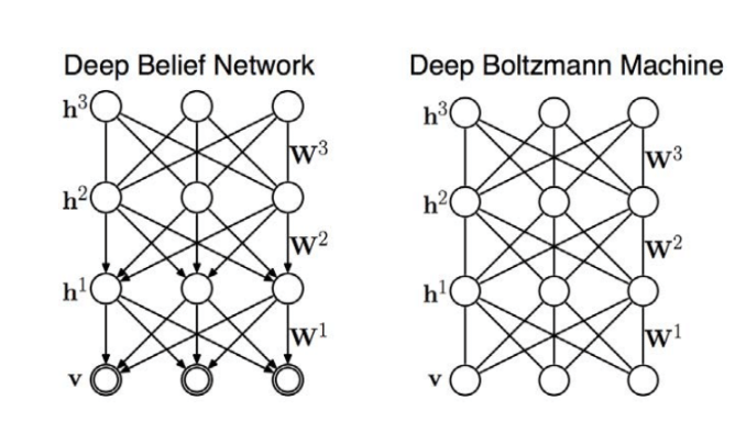
• Deep belief networks (DBNs)
  • Hybrid graphical model
  • Inference in DBNs is problematic due to explaining away
• Deep Boltzmann Machines (DBMs)

  • Undirected model

    

• Variational autoencoders (VAEs)

  Neural Variational Inference and Learning (NVIL)

  In fact, what VAE is doing is very similar to Helmholtz machine. For both there is a generative model and a inference model. Helmholtz machine directly solves the inference model using wake-sleep algorithm, while VAE introduces another technique to simplify the procedure so that you don?t have to solve the second relaxation. It is still solving the same lower bound of the data likelihood, but you are going to constrain the inference model so that it is easier to solve. Not a new model but an inference algorithm.

• Generative adversarial networks (GANs)

  Instead of having explicit hidden variables and conditional distributions, it uses something fancier. To parts of GAN:

  • Stochastic noise $Z$ and $Z$ go through a deterministic transition $G$
  • A discriminator $D$ which qualifies the resultant samples, such that it wants the fake samples to be distinguished from true data.
• Generative moment matching networks (GMMNs)
• Autoregressive neural networks

Synonyms in the literature

Since people in research community, either intentionally or unconciously, always come up with new names for existing old stuff, so we make some clarifications here in order to help you link current knowledge to historical literatures of origins of these techniques.

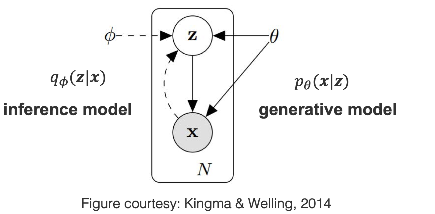
Inference model

The inference model refers to learn the posterior distribution. When estimating $p(X|Z)$ through the posterior distribution $p(Z|X)$, people can model $q(Z|X)$ to approximate the posterior, which is named as variational approximation (or variational inference). Synonyms of the inference model include

• Variational approximation
• Recognition model
• Inference network (if parameterized as neural networks)
• Recognition network (if parameterized as neural networks)
• (Probabilistic) encoder

Generative model

The generative model usually include prior + conditional (or joint), it is naturally understood as a likelihood model. Synonyms of the generative model include

• The (data) likelihood model
• Generative network (if parameterized as neural networks)
• Generator
• (Probabilistic) decoder

Note that encoder and decoder is a pair, usually correspond to “visible to latent” and “latent to visible”, respectively.

Recap of Variational Inference

Variational Lower Bound

Variational inference is a way to approximate the posterior $q(z|x)$ of a generative model. The approximation is defined variationally as a solution of an oprimization problem. Specifically, we define and maximize the lower bound for the log likelihood,

\begin{aligned} \log p(x) &= KL({q_{\phi}(z|x)}\,||\,{p_{\theta}(z|x)}) +\int_{z} q_{\phi}(z|x) \log \frac{p_{\theta}(z|x)}{q_{\phi}(z|x)}\\ &\geq\int_{z} q_{\phi}(z|x) \log \frac{p_{\theta}(z|x)}{q_{\phi}(z|x)}\\ &:= \mathcal{L}(\theta,\phi;x) \end{aligned}

which is also equivlent to mimizing the free energy

\[F(\theta,\phi;x)=-\log p(x)+ KL({q_{\phi}(z|x)}\,||\,{p_{\theta}(z|x)}).\]

Note that the KL divergence term in free energy will vanish if your approximation is equivalent to the true posterior.

Solve VI with EM

We can maximize the variational lower bound by EM steps. Specifically,

E-step: maximize $\mathcal{L}$ wrt. $\phi$, with $\theta$ fixed, i.e. \(\max_{\phi} \mathcal{L}(\theta,\phi;x)\)

Note that if closed form solutions exist, then it takes \(q_{\phi}^*(z|x)\propto \exp[\log p_{\theta}(x,z)].\)

M-step: maximize $\mathcal{L}$ wrt. $\theta$ with $\phi$, fixed, i.e. \(\max_{\theta} \mathcal{L}(\theta,\phi;x)\)

Variational inference for generative models are still considered numerically or algebrically difficult for many complex settings, and algorithms include Wake Sleep, VAEs, GANs, which we are going to introduce, are all relaxiation or surrogate of this.

Wake Sleep Algorithm

While the variational inference performs one relaxation to the true loss, Wake sleep algorithm performs one more relaxation. Recall that the free energy is

\[F(\theta,\phi;x)=-\log p(x)+ KL({q_{\phi}(z|x)}\,||\,{p_{\theta}(z|x)}).\]

Wake Phase

Wake Phase (correspond to the variational M step): minimize the free energy $F(\theta,\phi;x)$ wrt. $\theta$.

This equals to maximize the data likelihood

\[\max_{\theta} \mathbb{E}_{q_{\phi}(z|x)}\left[ \log p_{\theta}(x|z)\right].\]

Typically: we get samples from $q_{\phi}(z|x)$ through inference on hidden variables, then use them as targets for updating the generative model $p_{\theta}(z|x)$. This is named as a Wake Phase since we know $x$ and condition on the distribution of $x$ to draw samples.

Sleep Phase

Sleep Phase (correspond to the variational E step): minimize the free energy $F(\theta,\phi;x)$ wrt. $\phi$.

\[\max_{\phi}\mathbb{E}_{q_{\phi}(z|x)}\left[ \log p_{\theta}(x|z)\right]\]

While the Wake Phase simply involves a MLE estimation, however, the Sleep Phase runs into some difficulties since the parameter $\phi$ we are trying to maximizing with regard to is under the expectation, rather than originally in the term inside the expectation.

Either a sampling technique or a specific deterministic approximation step, there is a log term $\log p_{\theta}$ which has arbitrary scale and will lead to the negative effect of high variance. Then any mistake your model made in estimating $\theta$ will be amplified by the log term to get a large numerical value for the gradient of the update, which will further escalate the instability of your estimation.

To deal with this issue, Wake-Sleep use a new trick that inverts the direction of KL. So the free energy becomes,

\[F(\theta,\phi;x)=-\log p(x)+ KL( {p_{\theta}(z|x)} \,||\, {q_{\phi}(z|x)} ),\]

then we can alternatively mazimize

\[\max_{\phi}\mathbb{E}_{p_{\theta}(z,x)}\left[ \log q_{\phi}(z|x) \right].\]

We need to “Dreaming” up samples from $p_{\theta}(x|z)$ through top-down pass, then use them as targets for updating the inference model.

VI v.s. Wake-Sleep

Here is a comparision of variational inference and Wake Sleep algorithm:

Variational Inference v.s. Wake-Sleep

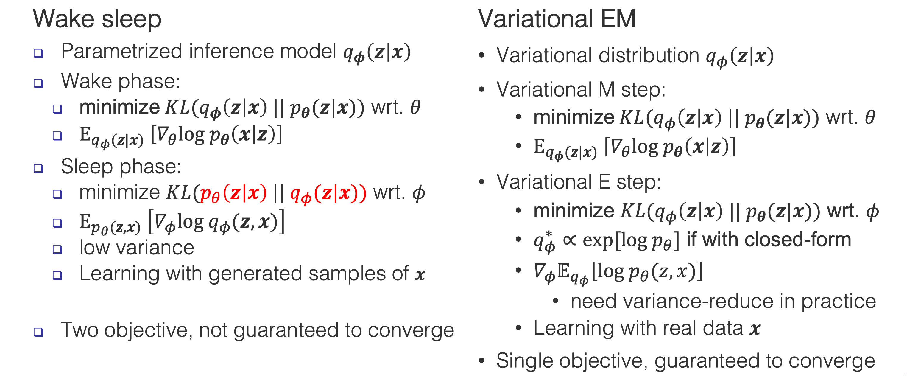
Note that Wake-Sleep is not guaranteed to converge, since inverting the two terms in KL has no theoratically gaurantee. You can consider Wake-Sleep as a heuristic algorithm.

Variational autoencoders

VAEs uses variational inference with an inference model, it is similar to Wake-Sleep but they differ in estimating the inference model. As we said before, its hard to estimate the inference model due to high variance of the gradient. Here, instead of changing the loss function (as the new trick of Wake-Sleep), the author of VAEs used reparameterization trick to reduce variance. Other alternatives for reducing variance include using control variates as in reinforcement learning:

• Variational Bayesian inference with stochastic search .
• Neural variational inference and learning in belief networks

Variational Auto-Encoders

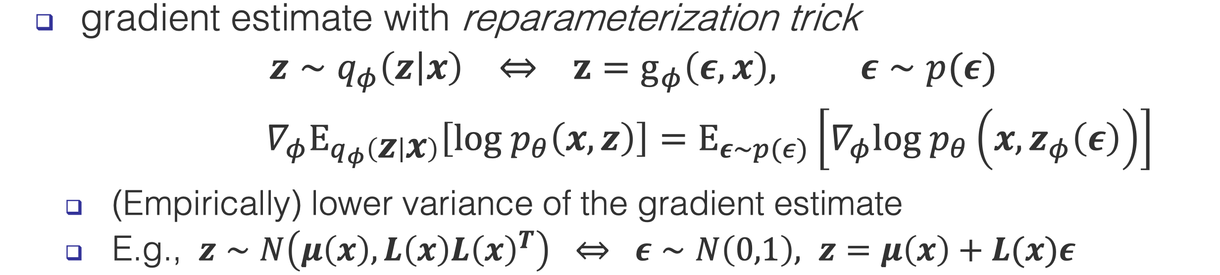
Reparameterization trick

Reparameterization trick assumes that the latent variables are resulted from a deterministic transformation of the inputs plus some noise. The deterministic transformation is a parameterization transformation that you can design, which makes calculating derivatives of everything much easier.

Reparameterization trick

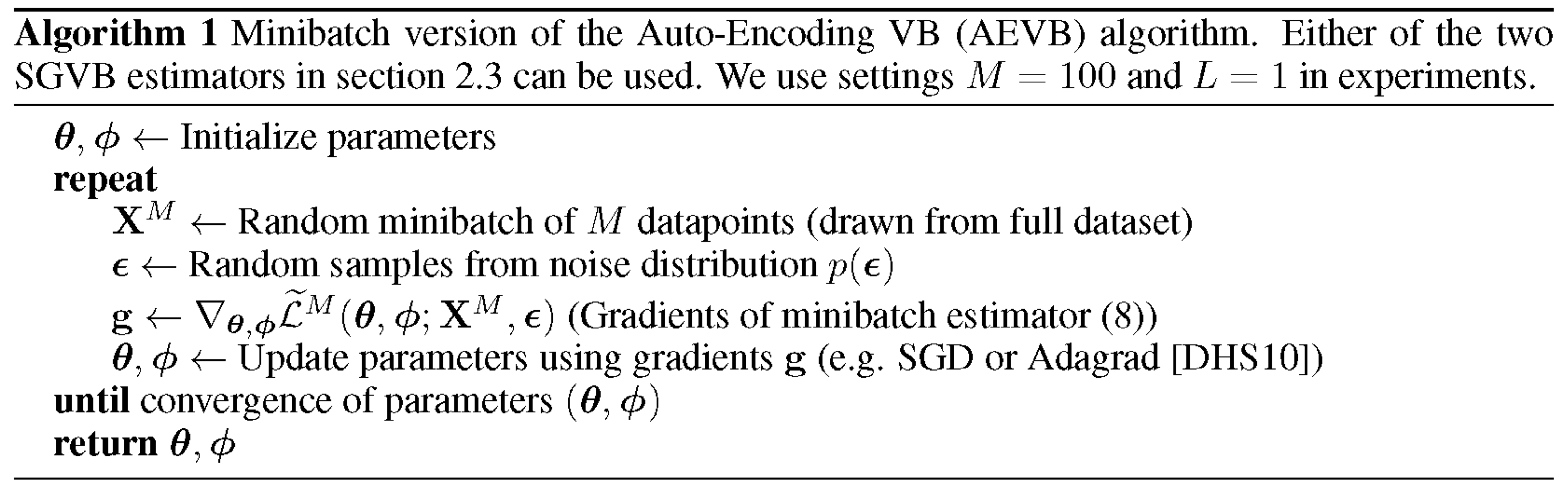
Algorithms

Reparameterization trick

Applications: Blurred Generations

• Computer Vision: Images generated by VAEs are always blurred due to the mode convering behavior, which is not favored. For eaxmple, celebrity faces generation

• Natural Langugae Processing: The blurred generation is favored in NLP since these blurred interpolation might some interesting outputs. Ambiguity is appreicated in languages but not in images

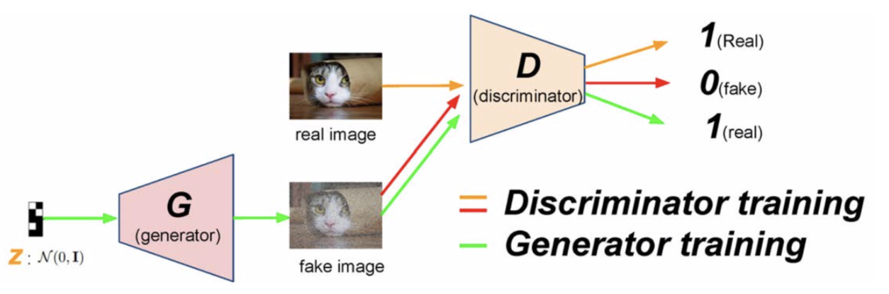
Generative adversarial networks

Generative adversarial networks (GANs) are composed of two models: the generative model (generator) and the discriminative model (discriminator). The generative model $G$ first samples latent variables $z$ from a prior distribution $p(z)$. Then it generates new data by $G_\theta(z)$ where $\theta$ are the parameters of the model. The discriminative model $D$ estimates the probability that a data $x$ came from the training data not from $G$. The figure below shows how GANs work.

GANs network

Learning GANs

The discriminator is trained to maximize the (log) probability of assigning correct labels to samples from the training dataset and samples generated from the generator. We use a cross-entropy-like objective function. This could be written as:

\[\max_D\mathcal{L}_D = \mathbb{E}_{\mathbf{x} \sim p_{data}(\mathbf{x})}[\log D(\mathbf{x})] + \mathbb{E}_{\mathbf{z} \sim p(\mathbf{z})}[\log (1-D(G(\mathbf{z})))]\]

The generator is trained to fool the discriminator, i.e., to minimize $\log(1-D(G(z))$. This can be written as:

\[\min_G\mathcal{L}_G = \mathbb{E}_{\mathbf{z} \sim p(\mathbf{z})}[\log (1-D(G(\mathbf{z})))]\]

In the early training phase where $G$ generates poor samples, this function saturates and thus it is hard to optimize with gradient descent. Therefore we use a equivalent problem instead that is:

\[\max_G\mathcal{L}_G = \mathbb{E}_{\mathbf{z} \sim p(\mathbf{z})}[\log D(G(\mathbf{z}))]\]

In short, learning GANs can be thought as a minimax game between the discriminator and the generator. Note that the generator defines an implicit distribution $p_{g_\theta}(\textbf{x})$. The minimax game described above has a global optimum at $p_{g_\theta}(\textbf{x}) = p_{data}(\textbf{x})$. In this case the discriminator cannot distinguish the two distributions, so

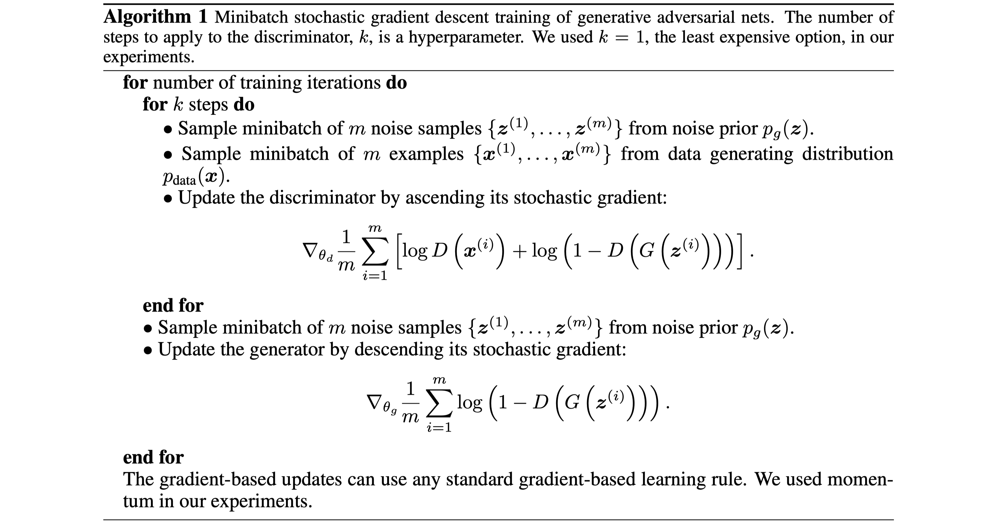
\[D(\textbf{x}) = \frac{p_{data}(\textbf{x})}{p_{data}(\textbf{x})+p_{g_\theta}(\textbf{x})} = \frac{1}{2}\]

An example of optimization of GANs using stochastic gradient descent from is shown below.

GANs training .

A unified view of deep generative models

For a unified view of deep generative models, we will reformulate GANs in the ‘variational-EM’ format. Let’s first define the conditional distribution of $\textbf{x}$ given $y$ as

p_\theta(\textbf{x}|y) = \begin{cases} p_{g_\theta}(\textbf{x}) & y=0 \quad \textrm{(generated data)} \\ p_{data}(\textbf{x}) & y=1 \quad \textrm{(training data)} \end{cases}

where $p_{g_\theta}(\textbf{x})$ is defined as $\textbf{x} \sim G_\theta(\textbf{z})$ where $\textbf{z} \sim p(\textbf{z}|y=0)$.

Define the discrimnator distribution $q_{\phi}(y|\textbf{x})$ where $\phi$ are parameters. Then the minimax problem of optimizing GANs formulates as

\[\max_{\phi}\mathcal{L}_\phi = \mathbb{E}_{p_\theta(\textbf{x}|y)p(y)}[\log q_\phi(y|\textbf{x})]\\ \max_{\theta}\mathcal{L}_\theta = \mathbb{E}_{p_\theta(\textbf{x}|y)p(y)}[\log (1-q_\phi(y|\textbf{x}))]\]

Gan v.s. Variational EM

Recall that in variational EM, we optimize one single objective

\[\mathcal{L}_{\boldsymbol{\phi},\boldsymbol{\theta} } = \mathbb{E}_{q_\boldsymbol{\phi}(\mathbf{z}|\mathbf{x})}[\log p_\boldsymbol{\theta}(\mathbf{x}|\mathbf{z})] +\mathrm{KL}(q_\boldsymbol{\phi}(\mathbf{z}|\mathbf{x})\parallel p(\mathbf{z}))\]

w.r.t to the inference parameter $\boldsymbol{\phi}$ and the generative parameter $\boldsymbol{\theta}$ alternately:

\[\max_\boldsymbol{\phi} \mathcal{L}_{\boldsymbol{\phi},\boldsymbol{\theta}}, \\ \max_\boldsymbol{\theta} \mathcal{L}_{\boldsymbol{\phi},\boldsymbol{\theta}}.\]

Now consider the above new formulation for GAN, objectives could be written

\[\max_\boldsymbol{\phi} \mathcal{L}_\boldsymbol{\phi} = \mathbb{E}_{p_\boldsymbol{\theta}(\mathbf{x}|y)p(y)}[\log q_\boldsymbol{\phi}(y|\mathbf{x})], \\ \max_\boldsymbol{\phi} \mathcal{L}_\boldsymbol{\theta} = \mathbb{E}_{p_\boldsymbol{\theta}(\mathbf{x}|y)p(y)}[\log q^\mathrm{r}_\boldsymbol{\phi}(y|\mathbf{x})].\]

Following the similar terms in variational EM, we could interpret the $q_\boldsymbol{\phi}(y|\mathbf{x})$ as the generative model and $p_\boldsymbol{\theta}(\mathbf{x}|y)$ as the inference model, since we are taking the expectation of $\log q_\boldsymbol{\phi}$ over $p_\boldsymbol{\theta}$, and now the $y$ is observed while the $\mathbf{x}$ is latent. In light of this, the $\mathbf{x}$ is the latent variable and and generation of $\mathbf{x}$ is the inference over $\mathbf{x}$.

In variational EM we minimize $-\log p(\mathbf{x}) + \mathrm{KL}(q_\boldsymbol{\phi}(\mathbf{z}|\mathbf{x})\parallel p_\boldsymbol{\theta}(\mathbf{z}|\mathbf{x}))$ so as to minimize the KLD from the inference model to the posterior. Also we could rewrite the objective of GAN in the form of minimizing KLD as that of variational EM. For each optimization step of $p_\boldsymbol{\theta}(\mathbf{x}|y)$ starting from an initial point $(\boldsymbol{\theta}_0, \boldsymbol{\phi}_0)$,

let $p(y)$ be a uniform prior distribution, and

\[p_{\boldsymbol{\theta}=\boldsymbol{\theta}_0}(\mathbf{x}) = \mathbb{E}_{p(y)}[p_{\boldsymbol{\theta}\\ =\boldsymbol{\theta}_0}(\mathbf{x}|y)], \\ q^\mathrm{r}(\mathbf{x}|y)\propto q^\mathrm{r}(y|\mathbf{x})p_{\boldsymbol{\theta}=\boldsymbol{\theta}_0}(\mathbf{x}),\]

we would have the equivalent update rule for $\boldsymbol{\theta}$ as in Lemma 1:

Lemma 1:

\begin{aligned} &\nabla_\boldsymbol{\theta} (-\mathbb{E}_{p_\boldsymbol{\theta}(\mathbf{x}|y)p(y)}[\log q^\mathrm{r}_{\boldsymbol{\phi}=\boldsymbol{\phi}_0}(y|\mathbf{x})])\mid_{\boldsymbol{\theta}=\boldsymbol{\theta}_0} \\ =&\nabla_\boldsymbol{\theta}(\mathbb{E}_{p(y)}[\mathrm{KL}(p_\boldsymbol{\theta}(\mathbf{x}|y)\parallel q^\mathrm{r}(\mathbf{x}|y))]-\mathrm{JSD}(p_\boldsymbol{\theta}(\mathbf{x}|y=0)\parallel p_\boldsymbol{\theta}(\mathbf{x}|y=1)))\mid_{\boldsymbol{\theta}=\boldsymbol{\theta}_0}. \end{aligned}

Here the generative model $p_\boldsymbol{\theta}(\mathbf{x}|y)$ becomes the variational approximation distribution for the posterior $q^\mathrm{r}(\mathbf{x}|y)$. We show that minimizing the KLD drives the generator $p_{g_\boldsymbol{\theta}}(\mathbf{x})$ to the true data distribution $p_\text{data}(\mathbf{x})$. For a uniform $y$ (being equally real or generated),

\[p_{\boldsymbol{\theta}=\boldsymbol{\theta}_0}(\mathbf{x}) = \mathbb{E}_{p(y)}[p_{\boldsymbol{\theta}=\boldsymbol{\theta}_0}(\mathbf{x}|y)] = {p_{g_{\boldsymbol{\theta}=\boldsymbol{\theta}_0}}(\mathbf{x}) + p_\text{data}(\mathbf{x})\over 2},\]

and thus we could break the KLD into two terms:

\begin{aligned} &\mathrm{KL}(p_\boldsymbol{\theta}(\mathbf{x}|y=1)\parallel q^\mathrm{r}(\mathbf{x}|y=1)) = \mathrm{KL}(p_\text{data}(\mathbf{x})\parallel q^\mathrm{r}(\mathbf{x}|y=1)) = \text{const.},\\ &\mathrm{KL}(p_\boldsymbol{\theta}(\mathbf{x}|y=0)\parallel q^\mathrm{r}(\mathbf{x}|y=0)) = \mathrm{KL}(p_{g_\boldsymbol{\theta}}(\mathbf{x})\parallel q^\mathrm{r}(\mathbf{x}|y=0)), \end{aligned}

where

\[q^\mathrm{r}(\mathbf{x}|y=0)\propto q^\mathrm{r}(y=0|\mathbf{x})p_{\boldsymbol{\theta}=\boldsymbol{\theta}_0}(\mathbf{x})\]

could be seen as a mixture of $p_{g_\boldsymbol{\theta}}(\mathbf{x})$ and $p_\text{data}(\mathbf{x})$ weighted by $q^\mathrm{r}(y=0|\mathbf{x})$. During the update we are drving the generator $p_{g_\boldsymbol{\theta}}(\mathbf{x})$ towards $q^\mathrm{r}(\mathbf{x}|y=0)$ by minimizing the KLD, thus driving it towards the thue distribution $p_\text{data}(\mathbf{x})$, as shown below.

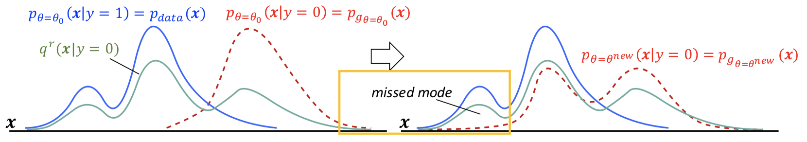
This KLD formulation allow GAN to recover the major modes, while also lead GAN to miss some minor modes of $p_\text{data}(\mathbf{x})$, where $p_{g_\boldsymbol{\theta}}(\mathbf{x})$ and $q^\mathrm{r}(\mathbf{x}|y=0)$ are small and already give a small KLD.

GAN v.s. VAE

Recap the VAE objective

Similar to GAN, we assum accordingly a perfect discriminator $q_{\star}(y|\mathbf{x})$ telling whether $\mathbf{x}$ is real or generated, and $q_{\star}^\mathrm{r}(y|\mathbf{x}) = q_{\star}(1-y|\mathbf{x})$, noticing that here $q_*$ is degenerate since we are always generating fake $\mathbf{x}$. We could write $\mathcal{L}^\text{vae}_{\boldsymbol{\theta}, \boldsymbol{\eta}}$ as

where the posterior

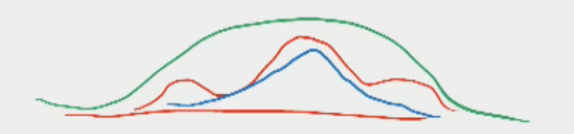
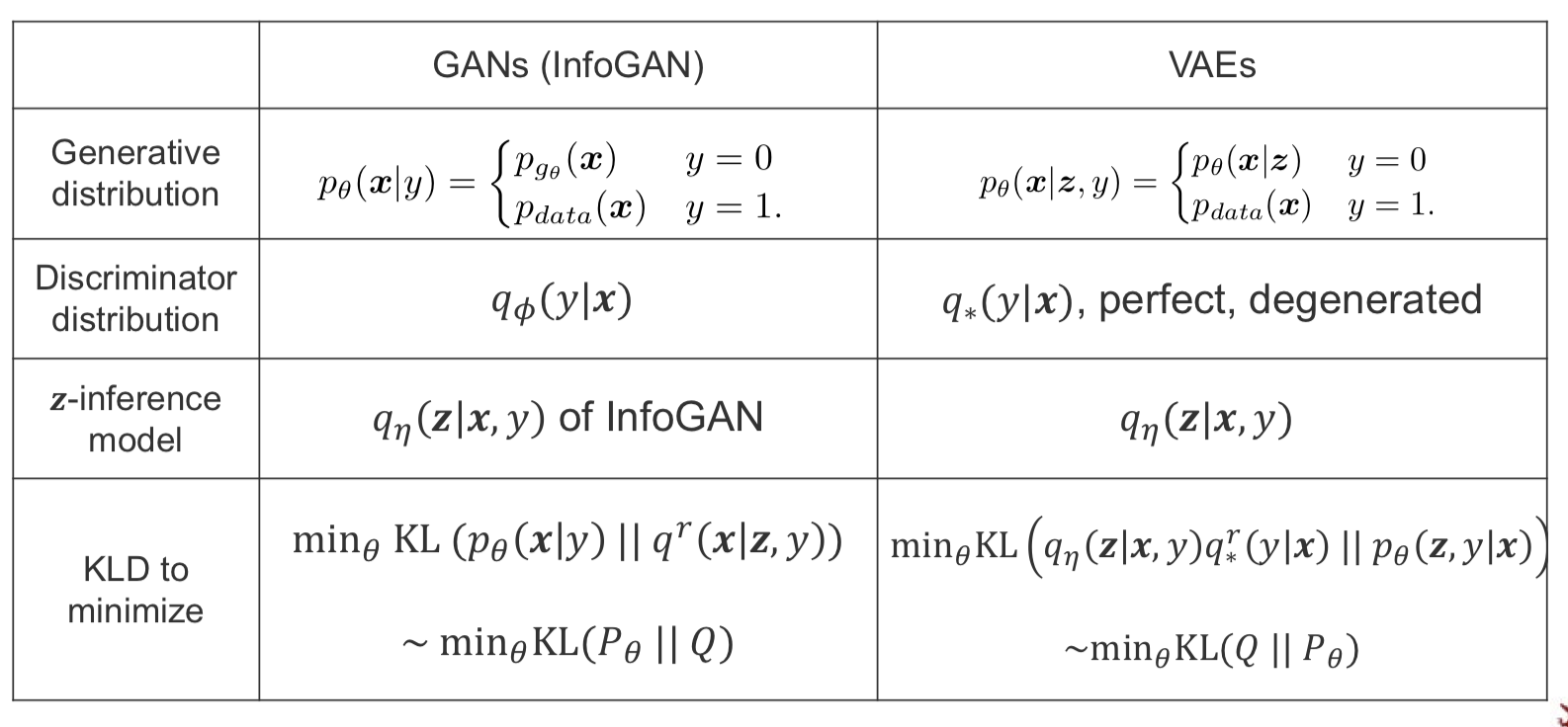
\[p_\boldsymbol{\theta}(\mathbf{z}|\mathbf{x},y) \propto p_\boldsymbol{\theta}(\mathbf{x}|\mathbf{z},y)p(\mathbf{z}|y)p(y)\]

is basically determined by the generative model $p_\boldsymbol{\theta}(\mathbf{z}|\mathbf{x},y)$ while the other two terms are fixed priors. In this way, VAE has the generative model on the right side of KLD, different to GAN. As shown below, GAN would provide a “sharp” distribution (blue curve)of covering major modes while missing minor modes of the true distribution (red curve) $p_\text{data}$, now VAE would provide a blurred distribution (green curve) to cover all the modes while less precisely covering area where $p_\text{data}$ is small.

The below table summarizes the comparion.

VAE/GAN v.s. Wake-Sleep

Look back at the wake-sleep algorithm:

\[\text{Wake}: \max_\boldsymbol{\theta} \mathbb{E}_{q_\boldsymbol{\lambda}(\mathbf{h}|\mathbf{x})p_\text{data}(\mathbf{x})}[\log p_\boldsymbol{\theta}(\mathbf{x}|\mathbf{h})], \\ \text{Sleep}: \max_\boldsymbol{\theta} \mathbb{E}_{p_\boldsymbol{\theta}(\mathbf{x}|\mathbf{h})p(\mathbf{h})}[\log q_\boldsymbol{\lambda}(\mathbf{h}|\mathbf{x})].\]

VAE only deals with the wake phase and extend it by also learning the inference parameter $\boldsymbol{\eta}$ (as in the KLD term in the original variational free energy):

\[\max_{\boldsymbol{\theta}, \boldsymbol{\eta}}\mathcal{L}^\text{VAE}_{\boldsymbol{\theta},\boldsymbol{\eta}}=\mathbb{E}_{q_\boldsymbol{\eta}(\mathbf{z}|\mathbf{x})p_\text{data}(\mathbf{x})}[\log p_\boldsymbol{\theta}(\mathbf{x}|\mathbf{z})]-\mathbb{E}_{p_\text{data}(\mathbf{x})}[\mathrm{KL}(q_\boldsymbol{\eta}(\mathbf{z}|\mathbf{x})\parallel p(\mathbf{z}))]\]

GAN only deals with the sleep phase and extend it by also learning the generative parameter $\boldsymbol{\theta}$:

\[\max_\boldsymbol{\phi} \mathcal{L}_\boldsymbol{\phi} = \mathbb{E}_{p_\boldsymbol{\theta}(\mathbf{x}|y)p(y)}[\log q_\boldsymbol{\phi}(y|\mathbf{x})], \\ \max_\boldsymbol{\phi} \mathcal{L}_\boldsymbol{\theta} = \mathbb{E}_{p_\boldsymbol{\theta}(\mathbf{x}|y)p(y)}[\log q^\mathrm{r}_\boldsymbol{\phi}(y|\mathbf{x})].\]