Lecture 18: Deep Generative Models (Part 2)

GANs and their variations, Normalizing Flows and Integrating domain knowledge in DL.

GANs and their variations

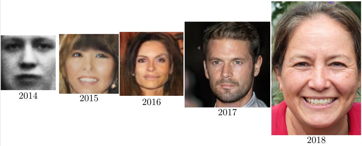
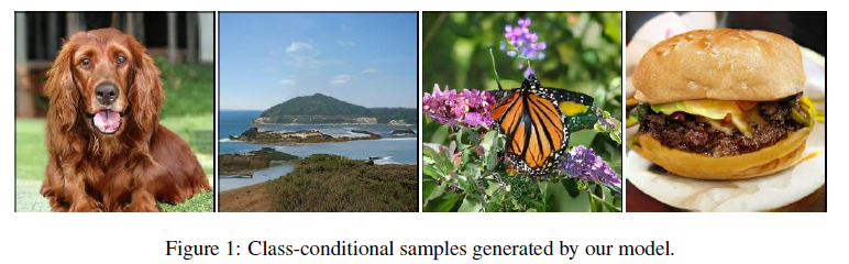
GAN Progress

Between 2014 and 2018, GAN has progressively been able to generate more high quality and more realistic images.

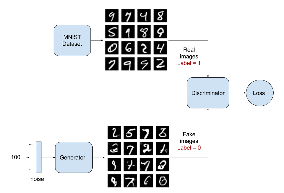
The changing of quality of image generation using GAN. Figure courtesy: Ian Goodfellow

Vanilla GAN Review

In the GAN setting, we have a generative model and a discriminator model. The generative model tries to generate new data given a prior, while the discriminative model distinguishes the difference between the generated data and the true data.

The generative part of GAN model maps a random noise to a generated data, i.e. $\bm{x} = G_\theta(\bm{z}), \bm{z} \sim p(\bm{z})$, where $z$ is a random noise and $x$ is the data space. It defines an implicit distribution over $x: p_{g_\theta}(x)$, and uses a stochastic process to simulate data $x$. It is intractable to evaluate the likelihood of the generated data.

The discriminative part of GAN tells apart the true data distribution from the generated distribution. Specifically, the discriminator $D_\phi (x)$ outputs a probability of $x$ being the true data.

The learning objective of GAN can be formulated as a minimax game between the generator and the discriminator. It simultaneously trains a discriminator $D$ to maximize the probability of assigning the correct label to both training examples and generated samples, and trains a generator $G$ to fool the discriminator.

\min_{G} \max _{D} V(D, G)=E_{\boldsymbol{x} \sim p_{\text { data }}(\boldsymbol{x})}[\log D(\boldsymbol{x})]+ E_{\boldsymbol{z} \sim p_{\boldsymbol{z}}(\boldsymbol{z})}[\log (1-D(G(\boldsymbol{z})))]

Example:

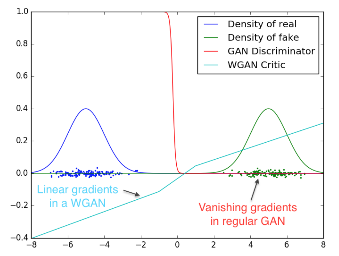
Wasserstein GAN (WGAN)

In the setting of vanilla GAN, if the data and model’s manifold are different, there can be negligible intersection between the two in practice. In this case, the loss function and gradients may not be continous or well-behaved. For example, for some $x$ such that $P_g(x)=0$ but $P_d(x) > 0$, KL divergence is infinite.

In order to solve the problem, WGAN was proposed, in which a new objective was used by changing the distance function to Wasserstein Distance (Earth Mover). It measures the minimum transportation cost for making one pile of dirt in the shape of one probability distribution to the shape of the other distribution.

The hard part of learning objective is to ensure that $|D|_{L} \leq K$ K-Lipschitz continuous. In the paper, it uses gradient-clipping to ensure $D$ has the Lipschitz continuity, which was acknowledged by the author that it may be a terrible way to do so, but it is simple, yet still effective, and performs better the vanilla GAN.

W (p_d, p_g) = {1 \over K} \cdot sup_{\|D\|_{L} \leq K} E_{x \sim p_d}[D(x)] - E_{x \sim p_g}[D(x)]

During training, we compare the GAN discriminator with the WGAN critic when learning to differentiate between two Gaussians. As we can see, the traditional GAN discriminator saturates and results in vanishing gradients, whereas WGAN critic provides very clean gradients on all parts of the space.

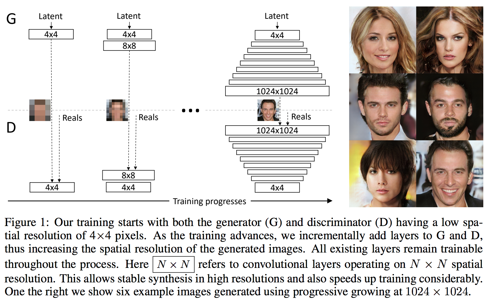
Progressive GAN

Although GAN can produce sharp images, in most cases, the images are in small resolutions with limited variation. Directly generating large image is impractical due to training instability. Due to those problems, the Progressive GAN was proposed to improve the training method for large images.

During the training phase, low resolution images were generated first, and then it progressively increases the resolution by adding new layers. The benefit of this training process is that the model could first detect large structure of image, and then shift its attention to finer details. The results are better generated images.

BigGAN

Similar to Progressive GAN, the BigGAN also targets at generating high fidelity, diverse images with models directly learned from data. The authors found that during the training process, GANs benefits dramatically from scaling. For example, in the paper, the model uses 2x–4x more parameters, and 8x larger batch size. To avoid the model collapse, a strong discriminator is used first, and then it is relaxed towards the end of training.

Normalizing Flows

Overview

Normalizing Flows transform a simple, usually factored distribution into a complex distribution through a sequence of smooth, invertible functions.

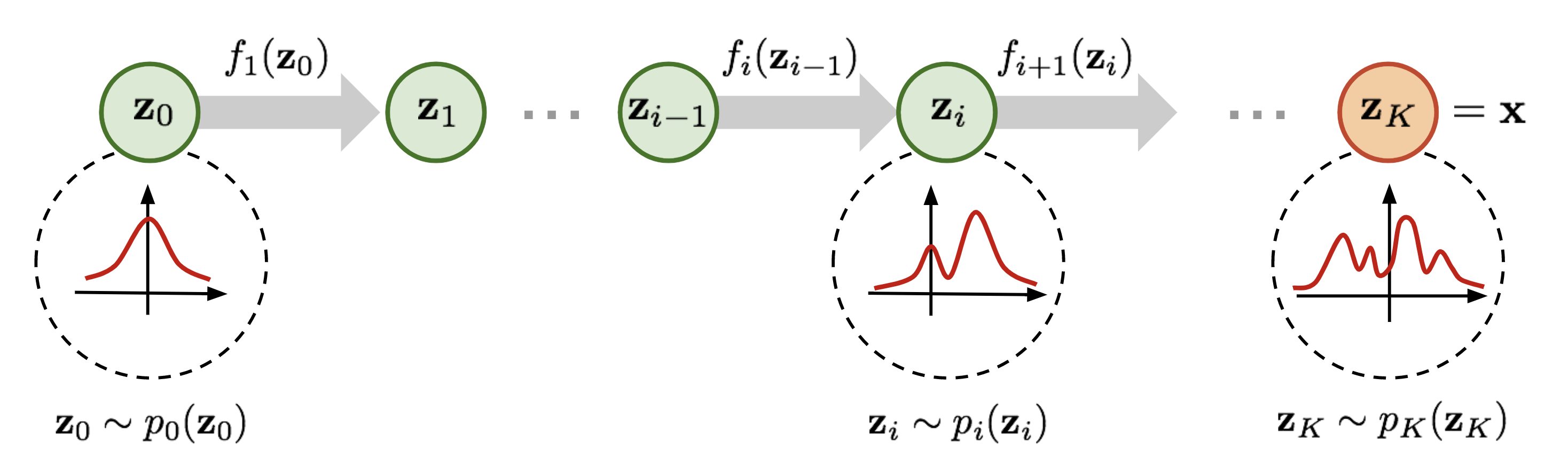
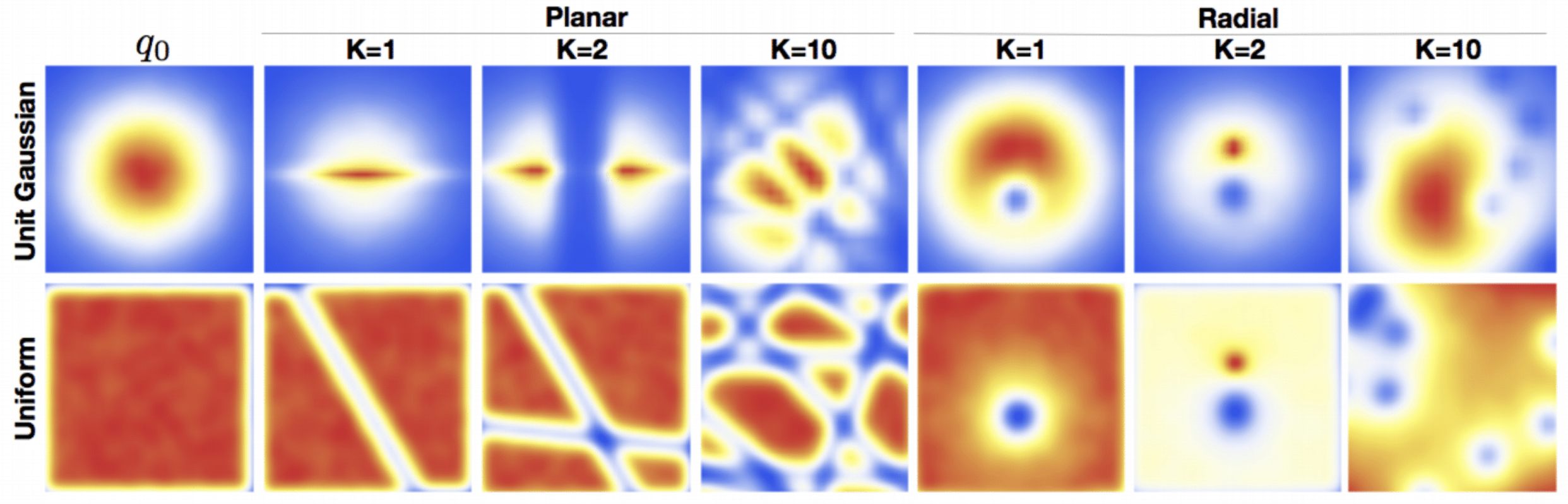
Transformation from a simple base distribution to a complex approximation to the true distribution. Figure courtesy: Lilian Weng

Example Density Transformations

Individual functions are restricted in architecture to ensure the tractability of the model. Such restrictions mean that each function alone is often quite simple, but a long sequence can result in arbitrarily complex target distributions.

Two different classes of transformations applied to 2-dimensional isotropic Gaussian and Uniform base distributions. Note the growth in complexity as the number of sequential function applications grows.

Benefits of Normalizing Flows:

Inference is Easy

The inference task is to learn the distribution of data, namely $p(x)$. From the training process, if we assume we know that $x = f(z)$, then $p(x) = p(z) \left|\det\frac{\partial f^{-1}}{\partial x}\right| = p(z)\left|\det\frac{\partial f}{\partial z}\right|^{-1}$. Therefore, it is simple to obtain the distribution by applying the inverse transformation to input and evaluating the probability of the result with respect to the base distribution. The calculation is made possible by requiring the transformation of $f$ to be invertible and having a Jacobian with a tractable determinant. Under this condition, the architecture of $f$ is typically chosen to be autoregressive, which means the Jacobian will be triangular.

Sampling is Easy

In order to sample for the data distribution, we can first sample a random $z$ from the base distribution, and then push through the transformation $f(z)$. It is similar to VAE sampling from $q(z)$.

Trained by Maximizing Log-Likelihood

$\log p(x) = \log p(z_0) + \sum_{i=1}^K \log\left|\det\frac{dz_{i-1}}{dz_i}\right|$

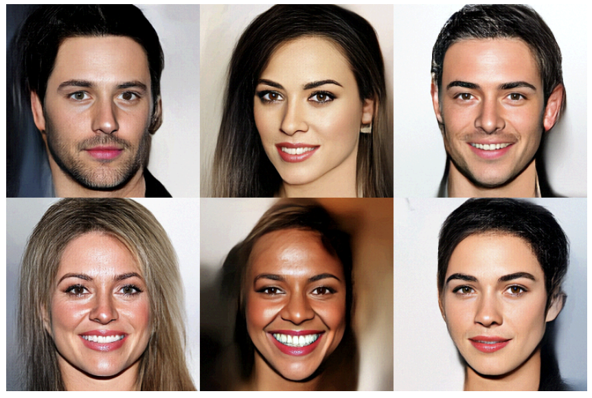
Current State of the Art: GLOW

The flow-based generative models are attractive due to its ability to perform exact hidden variable inference and tractable exact log-likelihood. GLOW builds off ideas of NICE and Real NVP, two of the first papers to use normalizing flows for deep generative modeling. Glow model generalizes the permutation operation of Real NVP with a 1x1 convolution of “channels”, and produces high-quality samples. The exact inference of hidden variable allows the generative model to learn meanful hidden representations, which could be used for disentangled image generations.

Integrating domain knowledge in DL

Integrating Domain Knowledge into Deep Learning

In recent years, deep learning has witnessed tremendous success in mulitple areas such as computer vision and natural language process. However, most deep neural network models usually rely on massive amount of labeled data, which are often expensive and hard to obtain. Furthermore, a common philosophy behind these machine learning success has been the use of end-to-end systems with minimally processed input features and minimally used domain knowledge. As a result, the models are hard to interpret and can’t take the advantage of any human expert domain knowledge. In order to improve the model when data is limited and expensive, or when we want to give more insights to the models, we have a motivation to incorporate human domain knowledge into the deep learning algorithms.

Deep generative models with learnable knowledge constraints

Deep generative models has been a powerful mechanism for learning data distribution and sampling, but most of the time people expect the model to uncover the underlying structure of massive training data, leaving valuable domain knowledge unused. The paper proposed a method for combining Posterior Regularization(PR) and Reinforcement Learning(RL) in order to utilize knowledge constraints to train deep neural nets.

deep generative model

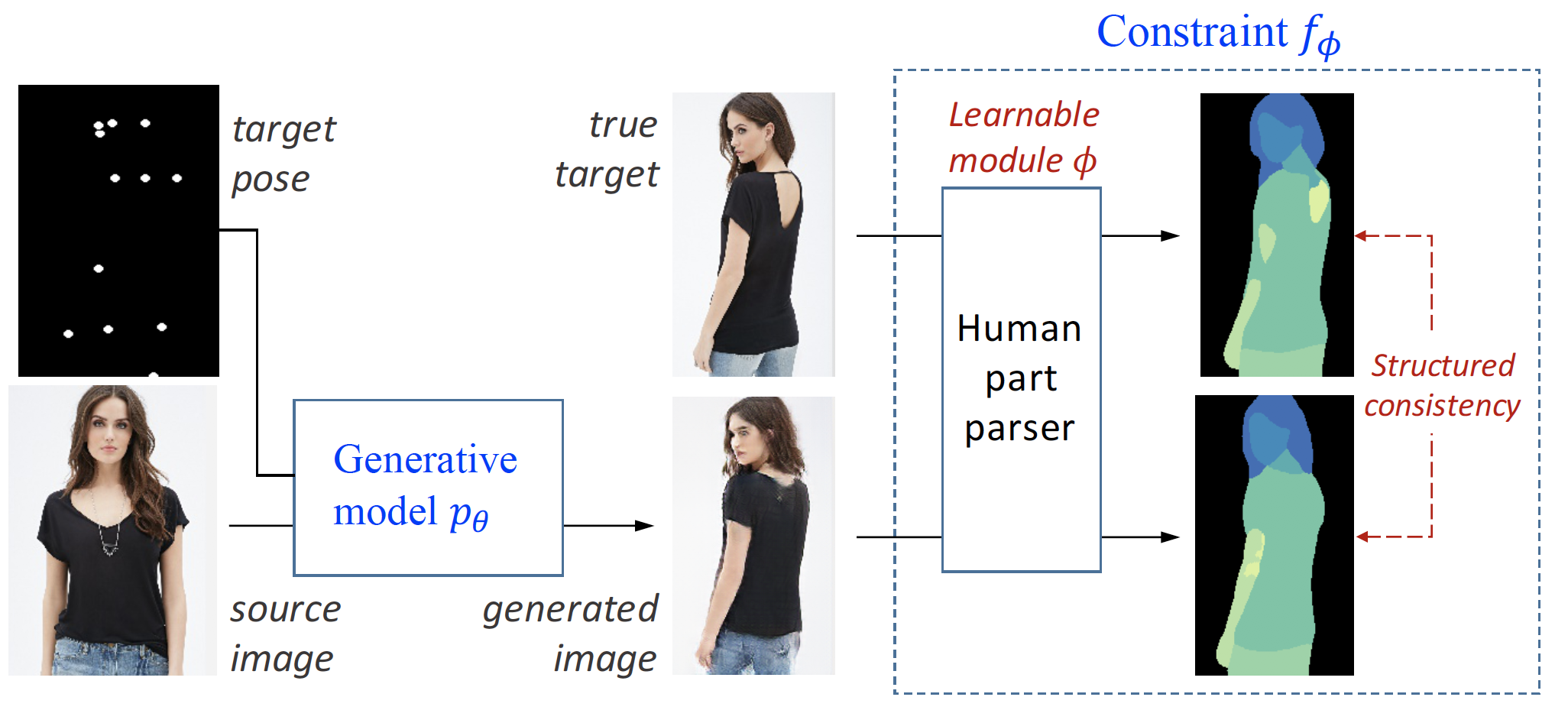
In the pose conditional person image generation task, we want to generate images based on some template of human poses. The input contains a human image and a target pose, which are minimally labeled dots indicating the target body position of person in the input image. We have a generative model $x\sim p_\theta(x)$, which is an implicit model that transforms the input source and pose directly to the pixels of generated image.

knowledge constraint

In order to evaluate the structural difference between the generated image and the target image, we introduce a constraint function $f_\theta(x)$ that encourages each of the body parts (e.g., head, legs) of the generated image to match the respective part of the target image. Specifically, the constraint $f_\theta(x)$ includes a human parsing module that classifies each pixel of a person image into possible body parts, and then evaluates cross entropies of the per-pixel part distributions between the generated and target images. The average negative cross entropy serves as the constraint score, and higher $f_\theta(x)$ values indicates a better generated $x$ in terms of pariticular domain knowledge.

learning objectives

In the previous sections, the proposed model has two parts: a deep generative model and a knowledge constraint model. In the optimization step, we should have a regular generative objective $\mathcal{L}(\theta)$, and a constraint regularization expectation $E_{p_\theta}[f(x)]$. Putting them together, the objective is simply:

\min_\theta \mathcal{L}(\theta) - \alpha E_{p_\theta}[f(x)]

In general, $E_{p_\theta}[f(x)]$ is hard to optimize unless $p_\theta$ is a GAN-like implicit generative model or an explicit distribution that can be efficiently reparametrized. For other models such as the large set of non-reparametrizable explicit distributions, the gradient $\nabla E_{p_\theta}[f_\theta(x)]$ is usually computed with the log-derivative trick and can suffer from high variance. For broad applicability and efficient optimization, PR instead imposes the constraint on an auxiliary variational distribution $q$, and introduces a KL divergence term:

\mathcal{L}(\theta,q)=KL(q(x) \| p_\theta(x)) - \alpha E_q[f(x)]

as proxy of $- E_{p_\theta}[f(x)]$

The optimization problem can be solve by EM algorithm:

In the E step, we optimize $\mathcal{L}(\theta,q)$ with respect to $q$ and get

q^*(x)=p_\theta(x)\exp\{\alpha f(x)\} / Z

where $Z$ is the normalization term.

In the M step, we plug in $q^*$ and optimize w.r.t. $\theta$ with:

\min_\theta KL(q(x)\|p_\theta(x))=\min_\theta \mathcal{L}(\theta) - E_{q^*}[\log p_\theta(x)]

Learnable constraints

In previous formulation, constraint $f(x)$ has to be fully-specified a priori and is fixed throughout the learning. It would be desirable or necessary to enable learnable constraint, so that people can specify the know constraints, while leaving the unknown parts learned by the model. We would like to introduce learnable parameters into the constraint function, such that we rewrite $f(x)$ as $f_\phi(x)$ where $\phi$ are learnable parameters. Learning $\phi$ is not straightforward, if we optimize $\phi$ in M-step, i.e. $\max_\phi E_{x\sim q(x)}[f_\phi(x)]$, such objective could be problematic due to the poor state of generative parameter $\theta$ at the initial stage. Instead, we can treat learning of constraint as an extrinsic reward motived by Reinforcement Learning, and get a joint learning algorithm for $\theta$ and $\phi$.

Learning with Constraints

Rule Knowledge Distillation

Knowledge distillation was first proposed as a way to compress (or distill) the knowledge of an ensemble of “teacher” neural networks into a single “student” network . This technique was motivated by two observations: (1) that ensemble methods tend to have better performance than their single-model counterpart, and (2) that deploying an ensemble of deep neural networks is not feasible at inference time (as every network needs to make a prediction).

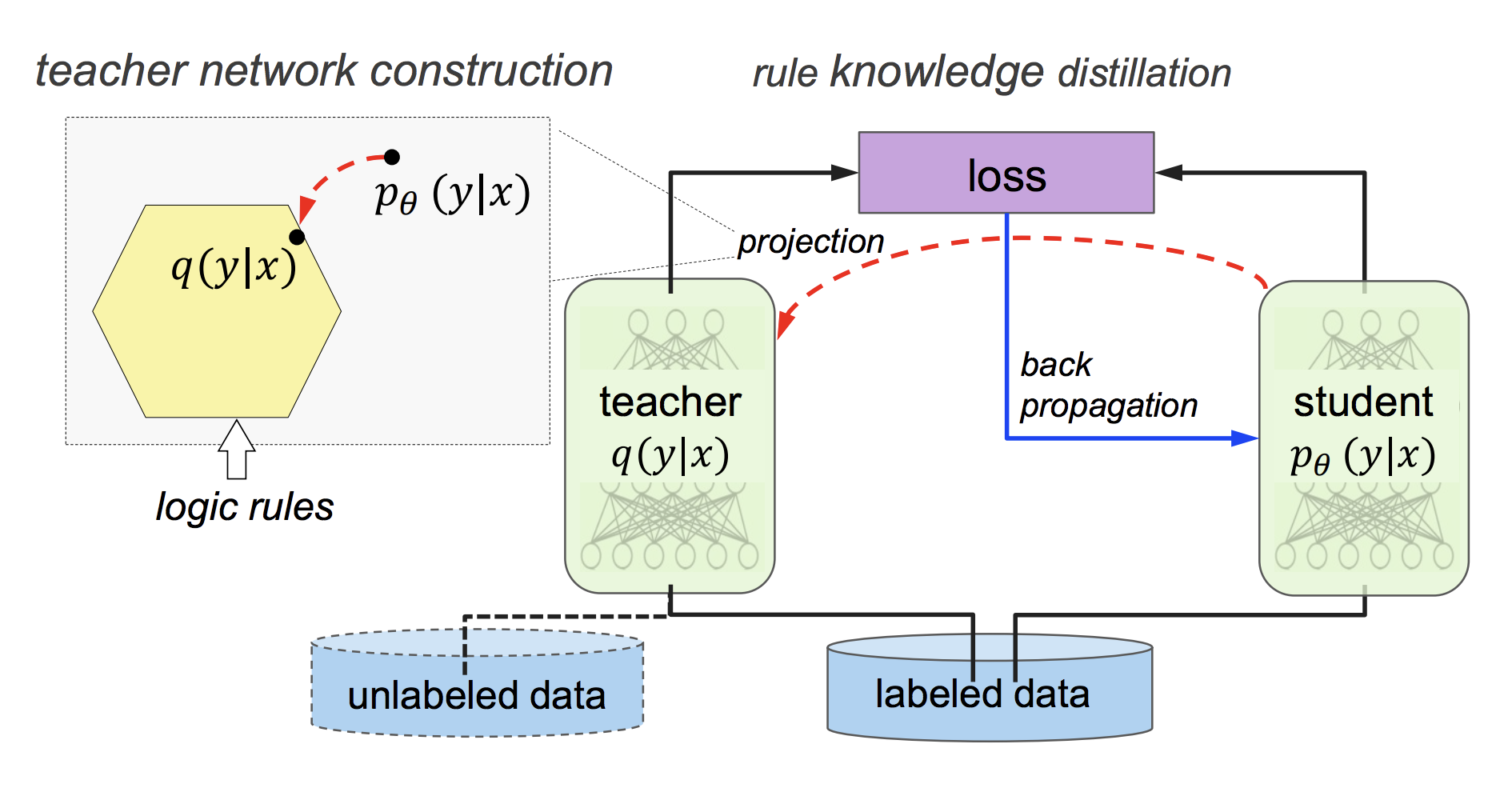
In the context of integrating domain knowledge into DL, a variant of knowledge distillation has been proposed as a way to have the student network learn “soft constraints” from a teacher network . Unlike the original variant, for this purposes we only need a single teacher that is, nevertheless, trained in parallel to the student.

Schematic view of the rule knowledge distillation technique proposed by .

For a multi-class prediction task, the Rule Knowledge Distillation technique works as follows:

A student network $p_{\theta}(y \mid x)$ parameterized by weights $\theta$ is trained to produce a prediction vector $\sigma_{\theta}(x)$.
At time step $t$, construct teacher network $q(y \mid x)$ by projecting $p_{\theta}(y \mid x)$ into a rule-regularized space. In other words, for a set of rules $(R_l, \lambda_l), l=1, …, L$ our goal is to find $q(y \mid x)$ such that, for every rule $l$ (specified using the soft logic in ), all rule groundings $r_{l, g_l}(X, Y), g=1, …, G_l$ are satisfied in expectation with confidence $\lambda_l$. More formally, we wish to solve the following optimization problem, \begin{aligned} \min_{q, \xi \geq 0} KL(q(Y \mid X) \mid \mid p_{\theta}(Y \mid X)) + C \sum_{l, g_l} \xi_{l, g_l} \\ \text{s.t.} \, \lambda_l (1 - E[r_{l, g_l}(X, Y)]) \leq \xi_{l, g_l} \\ g_l = 1, ..., G_l, l = 1, ..., L. \end{aligned}
where $\xi_{l, g_l}$ is a slack variable for each rule constraint and $C$ is a regularization parameter. Now, this problem has closed a form solution:
\begin{aligned} q^{\star}(Y \mid X) \propto p_{\theta}(Y \mid X) \exp{\left(-\sum_{l, g_l} C \lambda_l (1 - r_{l, g_l}(X, Y))\right)} \end{aligned}
Now, $p_{\theta}(y \mid x)$ is further trained to emulate the behavior of $q^{\star}$. This is achieved by reformulating the objective of $p_{\theta}(y \mid x)$ as \begin{aligned} \theta^{(t+1)} = \text{arg}\min_{theta} \frac{1}{N} \sum_{n=1}^N (1 - \pi) \ell(y_n, \sigma_\theta(x_n)) + \pi \ell(s_n, \sigma_\theta(x_n)) \end{aligned}
where $x_n, y_n, n=1, …, N)$ are the labeled training samples, $\ell$ is the loss function at hand and $s_n$ is the prediction of $q^{\star}$ at $x_n$. $\pi$ is an imitation parameter that calibrates the importance of the student network learning the hard labels $y_n$ vs. it imitating the behavior of $q^{\star}$. In , $\pi$ was set to $\pi^{(t)} = \min(\pi_0, 1-\alpha^t)$ for some lower bound $\pi_0 < 1$ and speed of decay $\alpha \leq 1$. This means that, at the beginning of training, $p$ is encouraged to learn the hard labels, behavior that eventually fades in favor of imitating $q^{\star}$.
Repeat the last two steps (alternating between training $q$ and refining $p$) until convergence.

As a final observation, notice that the second and third steps could be interpreted as the $E$ and $M$ steps in an $EM$ algorithm.

Incomplete or noisy domain knowledge

So far, domain knowledge has been specified through either a set of rules $(R_l, \lambda_l), l=1, …, L$, which require confidence parameters $\lambda_l$, or through a constraint function $f_{\phi}(x)$, which has to be constructed a priori (i.e., before training). Recent work, however, allows for more flexible specifications:

The work on learns the confidence parameters $\lambda_l$ for a given set of rules. This means that the knowledge encoded through these rules can be noisy, as the algorithm will learn to ignore false rules.
The work on allows for the constraint function $f_{\phi}(x)$ to have learnable components. These components are interpreted as the reward function in a reinforcement learning setting, meaning they can be learned using techniques from inverse reinforcement learning.