Lecture 19: Case Study: Text Generation
Introduction to text generation as a case study for deep learning and generative modeling.
Generating Natural Language
Language generation encompasses a wide range of tasks, including dialog system, machine translation, captioning, etc. The most common approach is to calculate the probability of the sentence as a product of the conditional probabilities over the sequence of tokens and use maximum likelihood estimation (MLE) to optimize the parameters:
\[\mathcal{L}_{\text{MLE}}(\theta) = \log{p(\mathbf{y}|\mathbf{x})} = \log{\prod_{t}{p(y_t|\mathbf{y}_{1:t-1}, \mathbf{x})}}.\]This widely used training paradigm, while practically effective, inevitably suffers from two fundamental problems:
- Exposure bias: The model is trained to generate the next word conditioned on the ground truth previous word sequence. However, at test time, the resulting model predicts an entire sequence one word at a time given the previous words generated by itself. The model is never exposed to the predictions of its own during training, and as a result the errors made along the way will quickly accumulate.
- Discrepancy between training objectives and evaluation metrics: The model is trained to maximize data log-likelihood but is evaluated using metrics like BLEU or ROUGE.
To bridge the gap between the training objective and test-time behavior, a reinforcement learning approach is proposed to maximize expected reward under the model distribution
At training time, the sequences are directly sampled from the model distribution $p_\theta(\mathbf{y})$, so that it has the potential to alleviate the exposure bias problem. Test-time evaluation metrics such as BLEU or ROUGE are used as reward funtion $R$, unifying the training objective and test-time usage.
However, due to the enormous space of possible word sequence, this method has high variance and poor exploration efficiency during training. Several works have been proposed to make the training efficient:
- Reward augmented maximum likelihood (RAML)
: Add reward-aware perturbation to the MLE data examples. - Softmax policy gradient (SPG)
: Use reward distribution for effective sampling and estimating policy gradient. - Data noising
: Add random noise to data.
Although seem different, these methods prove in another paper
Generalized Entropy Regularized Policy Optimization
The generalized ERPO objective is as follow:
\[\mathcal{L}(q, \theta) = \mathbb{E}_{q}{[R(\mathbf{y}, \mathbf{y}^*)]} - \alpha KL(q(\mathbf{y}|\mathbf{x}) | p_\theta(\mathbf{y}|\mathbf{x})) + \beta H(q),\]where $R$ is instantiated using BLUE or ROUGE, and $q$ is a variational distribution. The basic intuition is:
- We impose supervision $R$ on $q$, so that $q$ is optimized to gain more rewards.
- The KL divergence enforces model $p$ to stay close to the variational distribution $q$.
- Use additional entropy regularizer on $q$.
This objective could be solved using EM algorithm. For iteration $n$:
- In E-step, \(q^{n+1}(\mathbf{y} \mid \mathbf{x}) \propto \exp{\frac{\alpha \log{p_{\theta^n}(\mathbf{y} \mid \mathbf{x})} + R(\mathbf{y}, \mathbf{y}^{*})}{\alpha + \beta}}\)
- In M-step, \(\theta^{n+1} = \text{argmax}_{\theta}{\mathbb{E}_{q^{n+1}}{[\log{p_{\theta}(\mathbf{y} \mid \mathbf{x})}]}}\)
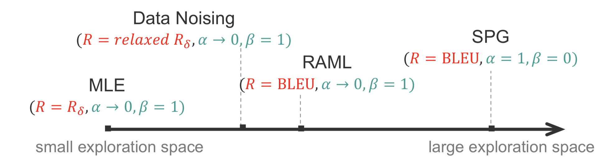
The intuition is that when $\alpha$ goes to infinity, $q$ completely follows previous strategy $p$; when $\beta$ goes to infinity, $q$ becomes uniform distribution. In the following section, we will show that MLE, Data Noising, RAML and SPG are special cases of the ERPO framework.
MLE, Data Noising, RAML and SPG as special cases of the ERPO framework
The ERPO framework has three key hyperparameters, the reward function $R$, $\alpha$ and $\beta$. In this section we show that popular RL algorithms can be retrieved from the ERPO framework by appropriately tuning those hyperparameters. We then use the ERPO interpretation of those algorithms in order to compare them. Finally we discuss how they can be integrated into a single algorithm under the umbrella of the ERPO framework.
MLE as a Special Case of ERPO
The $\delta$-reward is defined as:
\[R_\delta(\mathbf{y} |\mathbf{y}^*) = \begin{cases} 1 &\text{if } \mathbf{y} =\mathbf{y}^{*},\\ -\infty &\text{otherwise}. \end{cases}\]By setting $R=R_\delta$, $\alpha \to 0$ and $\beta=1$, the ERPO framework is reduced to the MLE estimation. Indeed, the corresponding the E-M steps are reduced to
- E-step: \(q(\mathbf{y} \mid \mathbf{x} )=\delta( \mathbf{y} = \mathbf{y}^{*})\)
- M-step:
The E-step corresponds to empirical data distribution while the M-step corresponds to maximum likelihood estimation.
Data Noising as a Special Case of ERPO
Data Noising can be thought as estimating the MLE of the data that is closed to the observed data. For that assume that $\mathcal{Y}$ is equipped with some metric $w$. Then we can retrieve the Data Noising approach from $ERPO$ by setting $\alpha \to 0$, $\beta=1$ and
\[R(y|y^*) = \begin{cases} 1 &\text{if } ||\mathbf{y} -\mathbf{y}^{*}||_w \leq \epsilon,\\ -\infty &\text{otherwise}. \end{cases}\]In the case that $\mathcal{Y}$ is discrete we may take $\epsilon$ to be a small natural number.
Reward Augmented Maximum Likelihood (RAML) as a Special Case of ERPO
For the rest of this section we let $R_c$ be a common reward function (in place of $R_c$ think of your favorite Gaussian Kernel). We can retrieve RAML by setting $R=R_c$,
$\alpha \to 0$ and $\beta=1$. In this case, the E-M steps are reduced to
- E-step: \(q(\mathbf{y} \mid \mathbf{x} ) \propto e^{R_c(\mathbf{y} ,\mathbf{y}^*)},\)
- M-step: \(\theta =\arg \max_\theta \mathbb{E}_q[ \log p_\theta(\mathbf{y} \mid \mathbf{x} )] = \arg \max_\theta \mathbb{E}_{\mathbf{y} \sim e^{R_c(\mathbf{y} ,\mathbf{y}^*)}}[ \log p_\theta(\mathbf{y} \mid \mathbf{x} )].\)
\(\mathbb{E}_{\mathbf{y} \sim e^{R_c(\mathbf{y} ,\mathbf{y}^{*})}}[ \log p_\theta(\mathbf{y} \mid \mathbf{x} )]\) is exactly the objective that RAML tries to maximize.
Softmax Policy Gradient as a Special Case of ERPO
By setting $\alpha=1, \beta=0$ and $R=R_c$ we can retrieve SPG. Indeed, in this case the E-M steps are reduced to
- E-step: \(q_{n+1}( \mathbf{y} \mid \mathbf{x} ) \propto p_{\theta^n}(\mathbf{y} \mid \mathbf{x} ) e^{R_c(\mathbf{y} ,\mathbf{y}^{*})},\)
- M-step: \(\theta^{n+1} =\arg \max_\theta \mathbb{E}_{q_{n+1}(\mathbf{y} \mid \mathbf{x} )}[ \log p_\theta(\mathbf{y} \mid \mathbf{x} )],\) which correspond to SPG.
Comparing MLE, Data Noising, RAML and SPG
First observe that all of MLE, Data Noising and RAML consists of a single execution of the E-M steps. MLE uses $R_\delta$. As a result it tremendously punishes any kind of exploration i.e.\@ considering any instances except the ones in the dataset. Following MLE, Data Noising allows for exploration only of points that are “closed” to the observed data.
RAML allows the whole exploration space. The data points that are closed to the observed data are more likely to be examine. However because it consists of a single execution of the E-M step it “does not have time” to integrate any new information and reconsider the probabilities according to which it observes new data.
Finally SPG allows for the whole exploration space. In addition the E-M steps are executed multiple times. As a result it integrates new information that is obtained by the exploration (here we are using the fact that $\alpha >0$). A data point that is examined at the $n^{th}$ iteration will potentially affect the shaping of $\theta^n$. As a result it will affect $q^{n+1}$ and thereafter which points should be “explored” in order to perform a Monte Carlo estimation at the M-step.
Interpolation Algorithm
In the above we saw that by choosing the proper reward function we can discourage (e.g. by setting $R=R_\delta$) or encourage (by setting $R=R_c$) exploration. Larger exploration space alleviates the exposure bias problem and yields better estimates. However algorithms with larger exploration space tend to converge slower, thus having to run for a longer period of time, since they explore more.
The interpolation algorithm tries to leverage the advantages of both, having a small and having a large exploration space. It exploits the natural idea of starting with a more restricted exploration space which gradually expands as time progresses. By varying the hyperparameters in the ERPO framework it starts by trying to estimate the MLE estimator. Then, as time progress it behaves more and more like $SPG$. Formally, in the Interpolation Algorithm, the $E$ step is substituted by \(q_{n+1}(\mathbf{y} |\mathbf{x} ) \propto \exp \bigg\{c\big(\lambda_{1,n+1} \log p_{\theta^n}(\mathbf{y} |\mathbf{x} ) + \lambda_{2,n+1} R_\delta(\mathbf{y}, \mathbf{y}^{*}) +\lambda_{3,n+1} R_c(\mathbf{y} ,\mathbf{y}^{*}) \big)\bigg\},\) where $0\leq \lambda_{1,n+1}, \lambda_{2,n+1}, \lambda_{3,n+1}$ and $\lambda_{1,n+1}+\lambda_{2,n+1}+\lambda_{3,n+1}\leq 1$. As $n$ increases $\lambda_{1,n+1}$ and $\lambda_{3,n+1}$ are increased while $\lambda_{2,n+1}$ is decreased.
Conditional Generation
The goal is to generate text that contains desired information infered from inputs. How we generate text depends on the amount of data for the task. When the training data is sufficient, we can use end-to-end training (i.e. sequence-to-sequence models, transformers, etc.).
Examples (# training examples)
- Machine Translation (10s of millions)
- Data Description (10s of thousands)
However for certain tasks, we do not have enough data for supervised trainings.
Examples:
- Attribute control
- Conversation control
In such cases, we consider controlled text generation in an unsupervised setting.
Text attribute transfer
The goal is to modify attribute values (ex. sentinment, tense) while keeping all other aspects unchanged
E.g., transfer sentiment from negative to positive:
- Original: “It was super dry and had a weird taste to the entire slice.”
- Output: “It was super fresh and had a delicious taste to the entire slice.”
Set up
- original sentence $\mathbf{x}$,
- original attribute $\mathbf{a}_x$
- target sentence $\mathbf{y}$
- target attribute $\mathbf{a}_y$
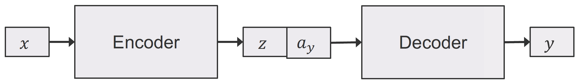
Task: $(\mathbf{x}, \mathbf{a}_y) \rightarrow \mathbf{y}$ where
- $\mathbf{y}$ has attribute $\mathbf{a}_y$
- $\mathbf{y}$ shares all attribute-independent properties of $\mathbf{x}$
Use encoder-decoder architecture to model: \(p_{\theta} (\mathbf{y} | \mathbf{x}, \mathbf{a}_y)\)
Sub-objectives
We jointly optimize two competing sub-objectives use cross-entropy loss. One for generating a sentence close to the original and another than ensure the sentiment of the generated sentence is correct (using a pretrained sentiment classifier).
- Auto-encoding loss:
- Classification loss:
Results
- Sentiment classification accuracy: 92%
- BLEU metric (measured against input sentence): 54
- LM perplexity: 239.8
Although the sentiment modification is successful (high classification accuracy) and the output sentence keeps similar non-attribute aspects as the original (BLEU score), the sentences do not make much sense (low perplexity). See the example below that shows the quality of genenerated sentences.
Solution: add language model (LM) as a discriminator with the objective $\max_{\theta} \text{LM}(\hat{\mathbf{y}})$
Results
- Sentiment classification accuracy: 91%
- BLEU metric: 57
- LM perplexity: 60.9
The generated sentences have similiar accuracy and BLEU scores but a much better perplexity. See example below.
- Original: “uncle george is very friendly to each guest”
- Output: “uncle george is very lackluster to each guest”
- with LM: “uncle george is very rude to each guest”
Text Content Manipulation
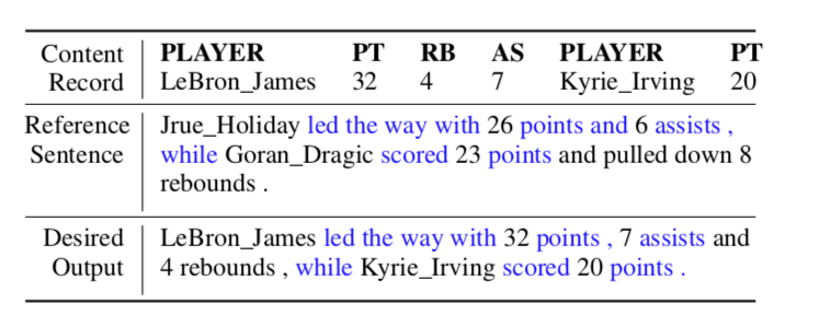
Another task is text content manipulation task, the goal of the task is to generate a new realistic sentence $\hat{\mathbf{y}}$that achieves (1) content fidelity by accurately describing the full content in x, and at the same time (2) style preservation by retaining as much of the writing style and characteristics of reference $y′$ as possible. The task is unsupervised as there is no ground-truth sentence for training. Below is a example,we want to rephrase the statistics of LeBron James and Irvine into a sentence in the style of the reference sentence “player 1 lead the way with blabla statitics while player 2 scored blabla..”.
There is no direct supervision data for this task. Similar to previous text attribute transfter task, we still use the keg idea proposed in
Model
Example training data and the model is shown below.
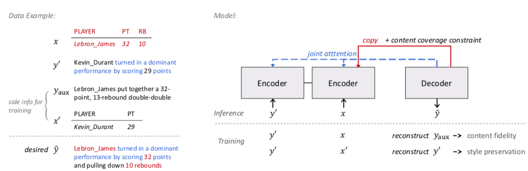
Let $p_{\theta}\left(\hat{\mathbf{y}} | \mathbf{x}, \mathbf{y}^{\prime}\right)$ denote the model that takes in a record $\mathbf{x}$ and a reference sentence $\mathbf{y}^{\prime}$ and generates an output sentence $\hat{\mathbf{y}}$ Here $\theta$ is the model parameter.
Competing Learning Objectives
Here we detail our two competitive sub-objectives. First we make use of the side information $(y_{aux}, x’)$ during training. Specifically, as the auxiliary sentence $y_{aux}$ was originally written by human to describe the content $x$ and thus can be seen to have the maximum data fidelity, we devise the first objective that reconstructs $y_{aux}$ given $(x, y’)$:
\[\mathbf{L}_{content}(\theta) = \log p_{\theta}(y_{aux} | x, y')\]This is content fidelity objective. The second goal is to preserve the style of reference $y’$, we want to encourage the model to generate sentences in a similar form of $y’$. We further notice that, if we feed the model with the reference sentence $y’$ and its corresponding record $x’$ (instead of $x$), the ground truth output of the case is indeed $y’$ itself (as $y’$ describes content $x’$, and is of course in the same style of itself). We thus can specify the second objective that reconstructs $y’$ given $(x’, y’)$:
\[\mathbf{L}_{style}(\theta) = \log p_{\theta}(y'|x',y')\]We call it the style preservation objective. The objective essentially treats the reference sentence encoder and the decoder together as an auto-encoding module, and effectively drives the model to absorb the characteristics of reference sentence and apply to the generated one.
The above two objectives are coupled together and train the model to achieve the desired goals:
\[\mathbf{L}_{joint}(\theta) = \lambda \mathbf{L}_{content}(\theta) + (1 − \lambda) \mathbf{L}_{style}(\theta)\]where $\lambda$ is the balancing parameter and gives us the ability to weight the two objectives.
Content Coverage Constraint
Generally the above model can achieve good performance but sometimes it can still not express the desired content accurately. So an additional learning constraint is devised based on the nature of content description—each data tuple in the content record should usually be mentioned exactly once in the generated sentence. This constraint on $x$ enables a simple yet effective way to encourage the behavior. Intuitively, we want each tuple to be copied once and only once on average. We thus minimize the following $L2$ constraint that drives the aggregated copy probability of each data tuple to be $1$:
\[\mathcal{C}(\boldsymbol{\theta})=\left\|\sum_{t} \mathbf{p}_{\mathbf{x}}^{(t)}-\mathbf{1}\right\|^{2}\]where $p(t)$ denotes the copy distribution over all data tuples at decoding step $t$.
Now the full training objective of the proposed model with the constraint is thus written as:
\[\mathcal{L}(\theta)=\mathcal{L}_{joint}(\theta)-\eta \cdot \mathcal{C}(\theta)\]where $\eta$ is the weight of the constraint.
Below is an example some sample output by this method and other methods
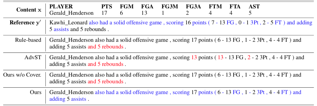
Text of erroneous content is highlighted in red, where […] indicates desired content is missing. Text portions in the reference sentences and the generated sentences by our model that fulfill the stylistic characteristics are highlighted in blue.
We can see that other methods tend to keep irrelevant content originally in the reference sentence (e.g., “and 5 rebounds” in the second case), or miss necessary information in the record (e.g., one of the player names was missed in the third case). The proposed model performs better in properly adding or deleting text portions for accurate content descriptions.
Below are some quantitive evaluation results and human evaluation results with other models
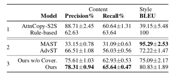
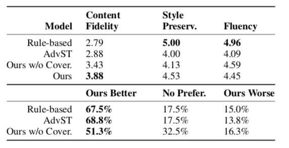
From the automatic evaluation results, we can find the model
Target-guided Open-domain Conversation
Target Guided conversation can be classified to the three classes below:
-
Task-oriented dialog: address a specific task, typically in close domain, e.g., service bot for booking a flight in the domain of flight service.
-
Open-domain chit-chat: improve user engagement, the conversation is random and hard to control, e.g., Apple Siri and Amazon Alex.
-
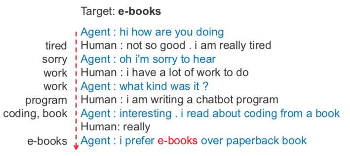
Target-guided conversation: something between the previous two tasks, the conversation is in open-domain and we want to control the conversation strategy to reach a desired topic in the end of conversation. It can bridge task-oriented dialog and open-domain chit-chat, e.g. conversational reccommender system, education, psychotherapy.
Here we discuss the target-guided conversation task, in this task we want our agents can start from any topic and reach a desired topic in the end of conversation with smooth and natural transitions. A successful example of target-guided conversation is shown below, we can see the agent can change the conversation topic from the starting “tired” to our final desired “e-books” with natural conversation and smooth transitions.
The challenge of open-domain target-guided conversation task is that there is no direct supervised data for the data, the conversation generation is totally unsupervised. To solve this challenge, we still use the previous idea, i.e, decompose the task into competitive sub-objectives and apply supervision methods on the sub-objectives. Partically, we have to achieve the subgoal of the conversation being natural and smooth and the subgoal that we reach the desired topic in the end. To make the conversation smooth and natural, we use chit-chat data to learn smooth single-turn transition; to reach desired target topic, we use rule-based multi-turn planning to restrict the agent to choose specific conversation topics at next step.
Here is a diagram showing how target-guided open-domain conversation agent works.
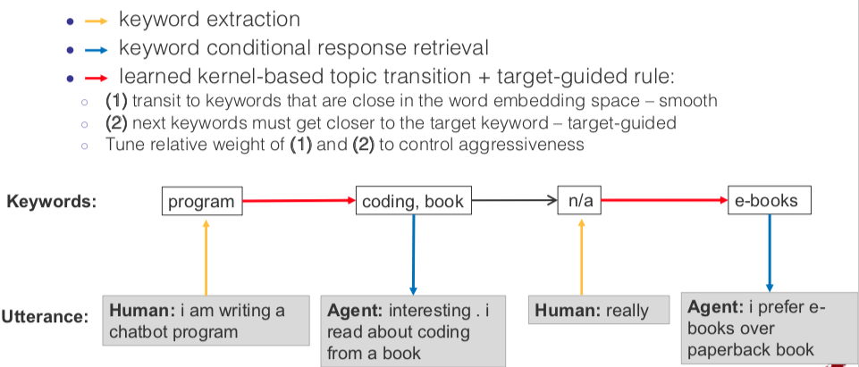
As the diagram shows, to achieve the open-domain target guided conversation. Given human utterance, we first extract the keyword(s) and then we use choose next conversation topic(s) based on learned kernel-based topic transition and target-guided rule, and then retrieve the conditional response for the next step conditioned on the keywords. When generating the keyword(s) for next step’s conversation topic(s), we can tune the relative weight of the two subgoals to control how relativly important to achieve smooth topic transition and to get closer to the keyword(s) of the target topic(s).
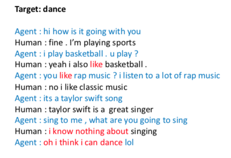
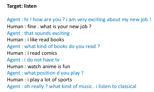
On the left of below is a successful example where the target topic is “dance” and we can see the transition is smooth and the conversation is natural. On the right is an example where the agent fails to change to the desired topic “listen”.
In summary, for the three tasks. We can decompose the task into competive sub-objectives and jointly train the sub-objectives with direct supervision.
Summary
We have two central goal for text generating tasks.
- Generating human-like, grammatical, and readable text I.e., generating natural language
-
Generating text that contains desired information inferred from inputs.
- Machine translation: Source sentence –> target sentence w/ the same meaning
- Data description: Table –> data report describing the table
- Attribute control: Sentiment: positive –> “I like this restaurant”
- Conversation control: Control conversation strategy and topic Source sentence –> target sentence w/ the same meaning
For supervised task where is plenty of supervised training data, we can use the sequence modelling to do end-to-end training, but for unsupervised tasks where there is no supervised data, we can decompose the task into competitive sub-objectives and train the sub-objectives with supervision.