Lecture 20: Reinforcement Learning & Control Through Inference in GM

Casting reinforcement learning as inference in a probabilistic graphical model.

Basic Concepts of Reinforcement Learning

Markov Decision Process:

Environment has a set of states $\mathcal{S}$.
Agent is given a set of possible actions $\mathcal{A}$.
Environment dynamics: transitions from state $s_t$ to a new state $s_{t+1}$ according to the transition probability $P\left(s_{t+1}|s_t, a_t\right)$ after the agent takes action $a_t$.
Reward function: $r(s,a) = \mathbb{E}[r_{t+1}|s_t = s, a_t = a]$ provides scalar rewards to the agent at each time step.
Trajectory of an agent: $\tau = (s_1, a_1, r_1, s_2, a_2, r_2, s_3, a_3, r_3, ...)$

What to do given a MDP:

Policy search: Find a policy $\pi: \mathcal{S} \to \mathcal{A}$ that outputs actions for each given state such that the cumulative reward along the trajectory is maximized.
Inverse RL: Given a set of optimal trajectories, infer the corresponding MDP.

Notations:

Returns:
- Return (cumulative reward) starting step $t$: $G_t = r_{t+1} + … + r_T$
- If $T = \infty$, we can use discounted return where $\gamma \in [0,1]$ is a discounted factor. Discounted reward is defined as $G_t = \sum_{k=0}^\infty \gamma^k r_{t+k+1} = r_{t+1} + \gamma G_{t+1}.$
Value function of a state $s$: $V_\pi(s) = \mathbb{E}[G_t \mid s_t = s] = \mathbb{E}_\pi\left[\sum_{k=0}^T \gamma^k r_{t+k+1} \mid s_t = s \right]$.
Q-Value of the state-action pair $(s,a)$: $Q_\pi (s,a) = \mathbb{E}_\pi \left[G_t \mid S_t = s, a_t = a \right] = \mathbb{E}_\pi \left[\sum_{k=0}^T \gamma^k r_{t+k+1} \mid s_t = s, a_t = a \right]$.

Bellman Equations:

Value function of a state $s$: $V_\pi(s) = \sum_a \pi(a \mid s) \sum_{s^\prime} p(s^\prime |s,a)[r(s,a) + \gamma \mathbb{E}_\pi [G_{t+1} \mid s_{t+1} = s']] = \sum_a \pi(a | s)\sum_{s^\prime} p(s^\prime | s,a) [r(s,a) + \gamma V_\pi(s^\prime)]$
Value fuction of a state-action pair $(s,a)$: $Q_\pi(s,a) = r(s,a) + \gamma \sum_{s^\prime} p(s^\prime,a) \sum_{a^\prime} \pi(a^\prime| s^\prime)Q_\pi(s^\prime, a^\prime)$

Optimal Policies:

Thus, we could define $\pi \geq \pi'$ if and only if $V_\pi(s) \geq V_{\pi^\prime}(s)$, for all $s \in \mathcal{S}$.
The optimal values of states are $V^*(s) = \max_\pi V_\pi(s) = \max_a \sum_{s^\prime} p(s^\prime \mid s,a)[r(s,a) + \gamma V^*(s^\prime)]$.
The optimal values of state-action pairs are $Q^*(s, a) = \max_\pi Q_\pi(s,a) = \sum_{s^\prime} p(s^\prime \mid s,a)[r(s,a) + \gamma \max_{a^\prime} Q^*(s^\prime, a^\prime)]$
Finally, an optimal policy is defined to be

\[\pi(a | s) = \delta (a = \arg \max_a Q^* (s, a))\]

and optimal trajectories are trajectories sampled from an optimal policy.

RL & Control as Inference in GM

This section introduces how RL and control can be seen through the lens of graphical models and inference in graphical models. The basic idea is to define a distribution over trajectories that are desired or optimal. A great resource for this is Sergey Levine’s tutorial on the same.

A Graphical Model for RL: the MDP as a PGM

Here we describe how a general MDP (Markov Decision Process) can be modeled as a probabilistic graphical model.

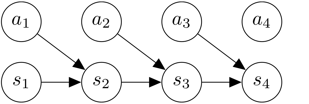
**MDP as a Graphical Model.** *Left*: Basic structure of GM of MDP. *Right*: GM conditioned on optimality variables (reward).

Consider the graphical model on the left. The state and action at every time step is modeled as a random variable in the graph. The graph is a chain-structure, Markovian DAG. The initial state is sampled according to some distribution $s_1 \sim p_1(s)$. Every state in the next time step depends on the previous state and previous action. This is called the dynamics of the environment, or the transition function: $s_{t+1} \sim p(s_{t+1} \mid s_t, a_t)$.

However, note that the selection of actions is kept very simple – it does not even depend on the state! Every action $a_t$ is sampled according to some fixed probability distribution. This is because, before specifying any reward function, we have a uniform prior over what actions should be taken. They are completely random for the time being.

\[\begin{aligned} &\text{Initial state }& &s_1 \sim p_1(s)\\ &\text{Transition }& &s_{t+1} \sim p(s_{t+1} \mid s_t, a_t)\\ &\text{Policy }& &a_t \sim \pi(a_t \mid s_t)\\ &\text{Reward }& &r_t = r(s_t, a_t) \end{aligned}\]

The unconditioned graphical models takes random actions, leading to sampling of random trajectories. In order to sample optimal trajectories based on a reward function, we need to somehow bake the reward function into the graphical model.

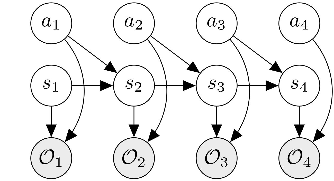
We do so by introducing optimality variables. The optimal variable $\mathcal{O}_t$ at timestep $t$ is a binary random variable which depends on $s_t$ and $a_t$. It is “true”, or takes the value 1 with probability $p(\mathcal{O}_t = 1 \mid s_t, a_t) = \exp(r(s_t, a_t))$. The higher the reward, the more likely it is that the optimality variable will be true.

\[{\color{red} \begin{aligned} &\text{Optimality }& &p(\mathcal{O}_t = 1 \mid s_t, a_t) = \text{exp}(r(s_t, a_t)) \end{aligned} }\]

So basically the reward $r_t$ is modeled as the log-probability of the optimality variable $\mathcal{O}_t$ being true. We will see how this helps recover the reinforcement learning objective when we do inference on this graphical model, while conditioning on all optimality variables being true.

The optimality variables are added to the graphical model on the right; you can see that the graphical model closely resembles an HMM, where the transition function is the same as that of the HMM, and the reward is captured through emission probabilities of optimality variables.

This models defines a probability distribution over trajectories. The advantage of this formulation is that it not only gives us optimal solution (trajectory), but also partially-optimal or almost-optimal solutions that are also associated with high rewards. Learning such stochastic behavior is helpful for smarter exploration and also from a transfer learning point of view.
Such a probabilistic model of the MDP provides a unified framework to ask different kinds of queries:
1. Infer optimal trajectories given rewards - $p(\tau \mid \mathcal{O}_{1:T})$, where $\tau = (s_1, a_1, …, s_T, a_T)$ is a trajectory.
2. Infer rewards and action priors given optimal trajectories (demonstrations). This is called inverse RL.
3. Infer policy given rewards $p(a_t \mid s_t, \mathcal{O}_{1:T})$. This is more closer to standard RL.

Distributions over optmial trajectories

In this section, we derive the distributions over trajectories $\tau$ conditioned on optimality variables $\mathcal{O}_t$ under the model defined in the previous section.

\[\newcommand{\opts}{\mathcal{O}_{1:T}} \newcommand{\opt}{\mathcal{O}} \begin{aligned} p(\tau \mid \opts) &\propto p(\tau, \opts)\\ &= p(s_1) \prod_{t=1}^T p(a_t \mid s_t)~p(s_{t+1} \mid s_t, a_t)~p(\opt_t \mid s_t, a_t)\\ &= p(s_1) \prod_{t=1}^T p(s_{t+1} \mid s_t, a_t)~\exp(r(s_t, a_t) + \log p(a_t \mid s_t))\\ &= \Bigg[ p(s_1) \prod_{t=1}^T p(s_{t+1} \mid s_t, a_t) \Bigg] \exp\Bigg(\underbrace{r(s_t, a_t)}_{\text{reward}} + \log \underbrace{p(a_t \mid s_t)}_{\text{action prior}} \Bigg) \end{aligned}\]

The action prior $p(a_t \mid s_t)$ is usually taken to be uniform, although it doesn’t have to be. For example, if we don’t want our agent to bump into walls, we can incorporate an appropriate action prior that prevents collisions into walls.

Inferring reward and prior that generate trajectory

To connect this formulation to more of what we have seen in PGMs, specifically CRFs, we consider the setting of inverse RL where given optimal trajectories executed by an optimal agent, we need to infer the best reward and priors that generate this trajectory.

The rewards and action priors are parametrized - they are linear functions of $\phi$ (and $\theta$) with features of the state (and action).

\[\newcommand{\opts}{\mathcal{O}_{1:T}} \newcommand{\opt}{\mathcal{O}} \begin{aligned} p(\tau \mid \opts) &\propto \Bigg[ p(s_1) \prod_{t=1}^T p(s_{t+1} \mid s_t, a_t) \Bigg] \exp\Bigg( r_{\textcolor{red}{\phi}}(s_t, a_t) + \log p_{\textcolor{red}{\theta}}(a_t \mid s_t) \Bigg)\\ &= \Bigg[ p(s_1) \prod_{t=1}^T p(s_{t+1} \mid s_t, a_t) \Bigg] \exp\Bigg(\textcolor{red}{\phi}^T \textbf{f}_r(s_t, a_t) + \textcolor{red}{\theta}^T \textbf{f}_p(s_t, a_t) \Bigg) \end{aligned}\]

The above formula looks like the featurized CRF, where the parameters can be learned using maximum likelihood estimation.

Optimal policy and planning via inference

Planning is taking actions in a state that provide the best possible future outcome. In this model, the optimal policy is defined as $p(a_t \mid s_t, \mathcal{O}_{t:T})$, i.e., the action to take given the current state, and conditioned on being optimal in all future time steps.

This reminds us of the HMM; we remarked above how the graphical model looks like an HMM. And we want to condition on emitted optimality variables in all future steps. Indeed analysis in this section will be similar to HMM, where we compute backward messages. The backward message $\beta_t$ is defined as

\[\begin{aligned} \textcolor{blue}{\beta_t(s_t, a_t)} &:= p(\mathcal{O}_{t:T} \mid s_t, a_t)\\ \textcolor{red}{\beta_t(s_t)} &:= p(\mathcal{O}_{t:T} \mid s_t) \end{aligned}\]

The recursion for backward messages can be obtained by expanding out $\beta_t(s_t, a_t)$ and $\beta_t(s_t)$.

\[\begin{aligned} \textcolor{red}{\beta_t(s_t, a_t)} &= p(\mathcal{O}_{t:T} \mid s_t, a_t)\\ &= \int_\mathcal{S} p(\mathcal{O}_{t:T}, s_{t+1} \mid s_t, a_t)~ds_{t+1}\\ &= \int_\mathcal{S} \underbrace{p(\mathcal{O}_{t:T} \mid s_{t+1})}_{\textcolor{blue}{\beta_{t+1}(s_{t+1})}}~p(s_{t+1} \mid s_t, a_t)~p(\mathcal{O}_t \mid s_t, a_t)~ds_{t+1}\\ &= p(\mathcal{O}_t \mid s_t, a_t)~\mathbb{E}_{s_{t+1} \sim p(s_{t+1} \mid s_t, a_t)} \Big[ \textcolor{blue}{\beta_{t+1}(s_t+1)} \Big]\\ \textcolor{blue}{\beta_t(s_t)} &= p(\mathcal{O}_{t:T} \mid s_t)\\ &= \int_{\mathcal{A}} p(\mathcal{O}_{t:T} \mid s_t, a_t)~p(a_t \mid s_t)~da_t\\ &= \mathbb{E}_{a_t \sim p(a_t \mid s_t)} \Big[ \textcolor{red}{\beta_t(s_t, a_t)} \Big] \end{aligned}\]

So the algorithm to compute backward messages is

\[\begin{aligned} \text{for } t &= T - 1 \text{ to } 1:\\ & \textcolor{red}{\beta_t(s_t, a_t)} = p(\mathcal{O}_t \mid s_t, a_t)~\mathbb{E}_{s_{t+1} \sim p(s_{t+1} \mid s_t, a_t)} \Big[ \textcolor{blue}{\beta_{t+1}(s_t+1)}\Big]\\ & \textcolor{blue}{\beta_t(s_t)} = \mathbb{E}_{a_t \sim p(a_t \mid s_t)} \Big[ \textcolor{red}{\beta_t(s_t, a_t)} \Big] \end{aligned}\]

Relating backward messages to RL

If we define

\[\begin{aligned} &V_t(s_t) = \log \textcolor{blue}{\beta_t(s_t)}\\ &Q_t(s_t, a_t) = \log \textcolor{red}{\beta_t(s_t, a_t)} \end{aligned}\]

and if we assume uniform action prior, then from the previous equations, we have

\[\begin{aligned} V_t(s_t) &= \log \int \exp(Q_t(s_t, a_t))~da_t\\ Q_t(s_t, a_t) &= r(s_t, a_t) + \log \mathbb{E}_{s_{t+1} \sim p(s_{t+1} \mid s_t, a_t)} \Big[ \exp(V_{t+1}(s_{t+1})) \Big] \end{aligned}\]

This is similar to the relationship between the Q-function and V-function in standard RL. Execpt that in the first equation, a log-integral-exponential approximates a max (also called “soft-max”). And in the second equation, the log-expectation-exponential is similar to a log-integral-exponential which is similar to a soft-max.

Let us carefully consider the recursive equation for $Q_t(s_t, a_t)$. For the case of deterministic dynamics, the expectation over $s_{t+1}$ reduces to a single evaluation over $s_{t+1}$, and we get $Q_t(s_t, a_t) = r(s_t, a_t) + V_{t+1}(s_{t+1})$. This is the same equation for deterministic dynamics of standard RL.

However, in general for stochastic dynamics, we end up taking the approximate max of $V(s_{t+1})$ over all $s_{t+1}$. That is, we end up being too “optimistic” about the transition. This is problematic because this results in learning risk-seeking behaviors where actions are chosen that may rarely lead to some states that are associated with high reward. We will see in the next section how such optimistic behavior can be addressed.

Optimal Policy

In the homework, we will show that the optimal policy is given by

\[\pi(a_t \mid s_t) = \frac{\beta_t(s_t, a_t)}{\beta_t(s_t)} = \exp \Big( Q_t(s_t, a_t) - V(s_t) \Big) = \exp(A_t(s_t, a_t)))\]

where $A_t(s_t, a_t)$ is known as the “advantage” function, since it denotes the advantage of taking action $a_t$ with respect to the “average” action for that state. There are two advantages of this form -

It has a natural interpretation, that better actions (which have high advantage) are more probable.
It facilitates random tie-breaking: if two actions have the same advantage - since the policy is stochastic, it samples them equally likely. Hence, this provides an automatic tie-breaking mechanism.
We can add a temperature parameter inside the exponent, which can either focus on sharp peaks (converging to a deterministic policy), or sample more uniformly (converging to a completely randomly policy).

Control via Variational Inference

Given this framework of inference for reinforcement learning with graphical models, one can ask the question about the relationship between the objective function the inference-basd policy is trying to optimize. In other words, what objective does inference optimize? We take a look at the KL divergence between trajectory distributions.

In the case for deterministic dynamics, we can express the probability of an optimal trajectory $\tau$ as

\[p(\tau) \propto \left[ p(\mathbf{s}_1) \prod_{t=1}^T p(\mathbf{s}_{t+1} | \mathbf{s}_t \mathbf{a}_t) \right] \exp \left( \sum_{t=1}^T r(\mathbf{s}_t, \mathbf{a}_t) \right).\]

On the other hand, the inference-based policy produces the following probability of the trajectory $\tau$:

\[\hat{p}(\tau) \propto \mathbf{1}[p(\tau) \neq 0] \prod_{t=1}^T \pi(\mathbf{a}_t | \mathbf{s}_t).\]

Computing the KL divergence between these two distributions, we have

\begin{aligned} -D_{KL}(\hat{p}(\tau) || p(\tau)) &= \mathbb{E}_{\tau \sim \hat{p}(\tau)} \left[ \sum_{t=1}^T r(\mathbf{s}_t, \mathbf{a}_t) - \log \pi(\mathbf{a}_t | \mathbf{s}_t) \right] \\ &= \sum_{t=1}^T \mathbb{E}_{(\mathbf{s}_t, \mathbf{a}_t) \sim \hat{p}(\mathbf{s}_t, \mathbf{a}_t)}[r(\mathbf{s}_t, \mathbf{a}_t))] + \mathbb{E}_{\mathbf{s}_t \sim \hat{p}(\mathbf{s}_t) }[H(\pi(\mathbf{a}_t | \mathbf{s}_t))] \end{aligned}

where $H$ is the entropy. So the objective is to maximize this quantity – the first term being the expected return (which is a standard RL objective), and the second term being the entropy of the policy, which helps promote stochasticity for exploration.

Now that we have seen the objective for the deterministic dynamics, let us think about the stochastic case as well. For the deterministic case, we have $Q(\mathbf{s}_t , \mathbf{a}_t) = r(\mathbf{s}_t, \mathbf{a}_t) + V(\mathbf{s}_{t+1})$ while for stochastic dynamics we will have, $Q(\mathbf{s}_t , \mathbf{a}_t) = r(\mathbf{s}_t, \mathbf{a}_t) + \log \mathbb{E}_{\mathbf{s}_{t+1} \sim p(\mathbf{s}_{t+1} | \mathbf{s}_t, \mathbf{a}_t)} [\exp(V(\mathbf{s}_{t+1}))]$ where the value function for the second term is now an expectation over all possible next states according to the transition distribution $p$. The second term however is not desirable because this make the Q function to be “optimistic” – if any of the future states have a high reward regardless of the intermediary states that lead to there, the exponential term will favor that high-reward-state only and disregard all other states. This means that the agent may present risk-seeking behavior as long as it has some non-zero probability of obtaining a high reward at the end. In the end of optimizing this objective, we will not be sure if the policy learned was indeed good, or we just got lucky with the stochastic dynamics.

Another problem for the stochastic dynamics is that the optimized trajectory distribution becomes $\hat{p}(\tau) = p(\mathbf{s}_1 | \mathcal{O}_{1:T}) \prod_{t=1}^T p(\mathbf{s}_{t+1} | \mathbf{s}_t , \mathbf{a}_t, \mathcal{O}_{1:T}) p(\mathbf{a}_t | \mathbf{s}_t \mathcal{O}_{1:T})$ which means that now the transition probability also depends on the optimality. What this means is that the agent can control both the actions and the dynamics of the system to create optimal trajectories, which is not desirable. We want the transition probability to remain the same regardless of the optimality.

To address these two issues, we use variational inference. Basically the goal is to find a variational distribution

\[q(\mathbf{s}_{1:T}, \mathbf{a}_{1:T})\]

which approximates

\[p(\mathbf{s}_{1:T}, \mathbf{a}_{1:T} | \mathcal{O}_{1:T})\]

while keeping the transition probabilities independent from the optimality. So the graphical model now looks slightly different as the figure below.

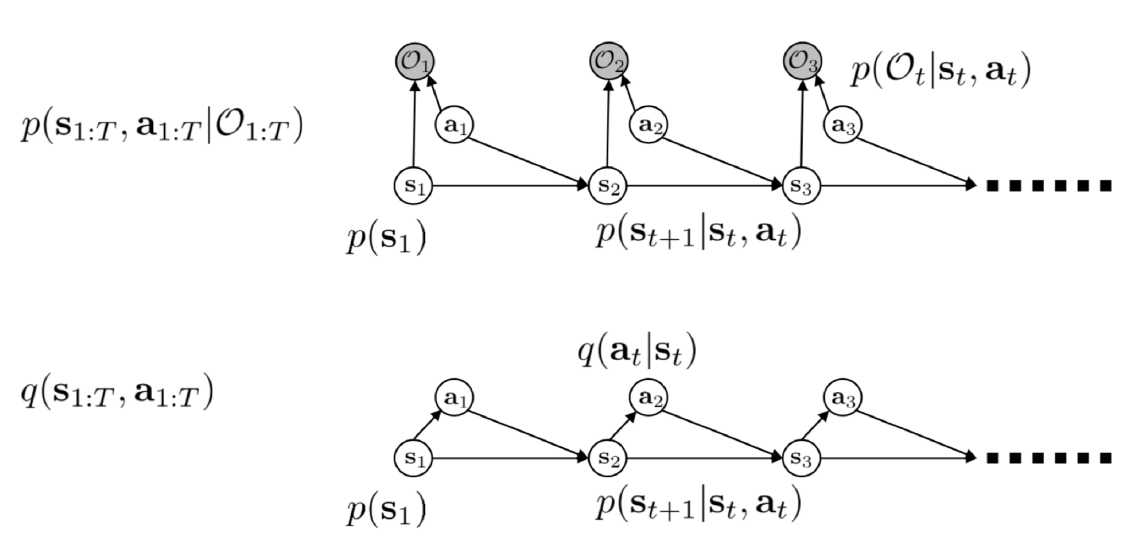
**Variational Inference for Stochastic Dynamics** Above is the original formulation of the trajectory distribution based on optimality, and using variational inference, we try to find a variational distribution(bottom) that approximates the original distribution without the optimality variable.

Following the figure, we let the probability of a trajectory produce by the policy as $q(\mathbf{s}_{1:T}, \mathbf{a}_{1:T}) = p(\mathbf{s}_1) \prod_{t=1}^T p(\mathbf{s}_{t+1} | \mathbf{s}_t , \mathbf{a}_t) q(\mathbf{a}_t | \mathbf{s}_t).$ where we introduce a variational policy term $q$ with the given stochastic dynamics.

Now using a standard approach in variational inference, we have the following ELBO:

\begin{aligned} \log p(\mathcal{O}_{1:T}) &= \log \int \int p(\mathcal{O}_{1:T}, \mathbf{s}_{1:T}, \mathbf{a}_{1:T}) d\mathbf{s}_{1:T} d\mathbf{a}_{1:T} \\ &= \log \int \int p(\mathcal{O}_{1:T}, \mathbf{s}_{1:T}, \mathbf{a}_{1:T}) \frac{q(\mathbf{s}_{1:T}, \mathbf{a}_{1:T})}{q(\mathbf{s}_{1:T}, \mathbf{a}_{1:T})} d\mathbf{s}_{1:T} d\mathbf{a}_{1:T} \\ &= \log \mathbb{E}_{(\mathbf{s}_{1:T}, \mathbf{a}_{1:T}) \sim q(\mathbf{s}_{1:T}, \mathbf{a}_{1:T})}\left[ \frac{p(\mathcal{O}_{1:T}, \mathbf{s}_{1:T}, \mathbf{a}_{1:T})}{q(\mathbf{s}_{1:T}, \mathbf{a}_{1:T})} \right] \\ &\geq \mathbb{E}_{(\mathbf{s}_{1:T}, \mathbf{a}_{1:T}) \sim q(\mathbf{s}_{1:T}, \mathbf{a}_{1:T})} [\log p(\mathcal{O}_{1:T}, \mathbf{s}_{1:T}, \mathbf{a}_{1:T}) - \log q(\mathbf{s}_{1:T}, \mathbf{a}_{1:T})] \\ &= \mathbb{E}_{\tau \sim q} \left[\sum_{t=1}^T r(\mathbf{s}_t, \mathbf{a}_t) - \log q(\mathbf{a}_t | \mathbf{s}_t ) \right] \\ &= \sum_{t=1}^T \mathbb{E}_{(\mathbf{s}_t, \mathbf{a}_t) \sim q} [r(\mathbf{s}_t, \mathbf{a}_t)] + H(q(\mathbf{a}_t | \mathbf{s}_t )) \end{aligned}

where the inequality follows from Jensen’s inequality. Now notice that the objective now is composed of two components just like the deterministic case, but in terms of the variational distribution. The first term is the expected return induced by the variational policy, and the second term is the entropy of the variational policy. Notice that this objective only allows the agent to modify the policy and not the dynamics, while keeping the overall form same as the deterministic case. So the stochastic case maximizes this ELBO in search for an optimal $q$.

Using the similar approach to the deterministic case, we obtain the following expressions for the Value function and the Q function, $V_t(\mathbf{s}_t) = \log \int \exp(Q_t(\mathbf{s}_t, \mathbf{a}_t)) d\mathbf{a}_t$

$Q_t(\mathbf{s}_t, \mathbf{a}_t) = r(\mathbf{s}_t, \mathbf{s}_a) + \mathbb{E}[V_{t+1}(\mathbf{s}_{t+1})]$ along with the expression for the variational policy $q(\mathbf{a}_t | \mathbf{s}_t) = \exp(Q(\mathbf{s}_t , \mathbf{a}_t) - V(\mathbf{s}_t)),$ but now with a guarantee that (1) the agent does not manipulate the dynamics of the system, and (2) the optimism introduced from previous framework is no longer an issue as the update on Q function does not involve exponent of values.