Lecture 21: Sequential decision making (part 2): The algorithms

An introduction for max-entropy RL algorithms

Recap: Control as Inference

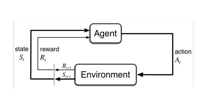
In Control setting:

Initial State $s_0 \sim p_0(s)$
Transition $s_{t+1} \sim p(s_{t+1} \mid s_t, a_t)$
Policy $a_{t+1} \sim \pi(a_t \mid s_t)$
Reward $r_t \sim r(s_t, a_t)$

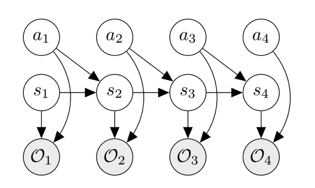
In Inference setting:

Initial State $s_0 \sim p_0(s)$
Transition $s_{t+1} \sim p(s_{t+1} \mid s_t, a_t)$
Policy $a_{t+1} \sim \pi(a_t \mid s_t)$
Reward $r_t \sim r(s_t, a_t)$
Optimality $p(\mathcal{O_t} = 1 \mid s_t, a_t) = exp(r(s_t, a_t))$

In the classical deterministic RL setup, we have:

\begin{aligned} & V_\pi(s) := \mathbb{E}_\pi \displaystyle \sum_{k=0}^T \left[\gamma^k r_{t+k+1} \mid s_t = s \right]\\ & Q_\pi (s, a) := \mathbb{E}_\pi \displaystyle \sum_{k=0}^T \left[\gamma^k r_{t+k+1} \mid s_t = s, a_t = a \right]\\ & \pi_*(a \mid s) := \delta(a = \underset{a}{\text{argmax}} Q_*(s,a))\\ \end{aligned}

Let $V_t(s_t) = \log \beta_t(s_t), Q_t(s_t, a_t) = \log \beta_t(s_t, a_t), V(s_t) = \log \int exp(Q(s_t, a_t) + \log p(a_t \mid s_t)) da_t$. Denote $\tau = (s_1,a_1, …, s_T,a_T)$ as the full trajectory. Denote $p(\tau) = p(\tau \mid \mathcal{O}_{1:T})$. Running inference in this GM allows us to compute:

\begin{aligned} & p(\tau \mid \mathcal{O}_{1:T}) \propto p(s_t) \displaystyle \prod_{t=2}^T p(s_{t+1} \mid s_t, a_t) \times exp(\displaystyle \sum_{t=1}^T r(s_t, a_t)) \\ & p(a_t \mid s_t, \mathcal{O}_{1:T}) \propto exp(Q_t(s_t, a_t) - V_t(s_t)) \\ \end{aligned}

From the perspective of control as inference, we optimize for the following objective:

\[-D_{KL}(\hat{p}(\tau) \mid\mid p(\tau)) = \sum_{t=1}^T \mathbb{E}_{(s_t, a_t) \sim \hat p(s_t, a_t)}\left[r(s_t, a_t)\right] + \mathbb{E}_{s_t \sim \hat{p}(s_t)}\left[\mathcal{H}(\pi(a_t \mid s_t))\right]\]

For deterministic dynamics, we get this objective directly.
For stochastic dynamics, we obtain it from the ELBO on the evidence.

Types of RL Algorithms

The objective of RL learning is to find the optimal parameter s.t. maximize the expected reward.

\[\theta^*=\arg\max_\theta \mathbb{E}_{\tau\sim p(\tau)}\left[\sum_{t=1}^T r(s_t,a_t)\right]\]

Policy gradients: directly optimize the above stochastic objective
Value-based: estimate V-function or Q-function of the optimal policy (no explicit policy; the policy is derived from the value function)
Actor-critic: estimate V-/Q-function under the current policy and use it toimprove the policy (not covered)
Model-based methods: not covered

Policy gradients

In policy gradient, we directly optimize the target expected reward w.r.t the policy $\pi_\theta$ itself.

\[\begin{aligned} J(\theta)&=\mathbb{E}_{\tau \sim p_{\theta}(\tau)}\left[\sum_{t=1}^{T} r\left(s_{t}, a_{t}\right)\right] \approx \frac{1}{N} \sum_{i=1}^{N} \sum_{t=1}^{T} r\left(s_{i, t}, a_{i, t}\right) \\ \nabla_{\theta} J(\theta) &=\nabla_{\theta} \mathbb{E}_{\tau \sim p_{\theta}(\tau)}[r(\tau)]=\int r(\tau) \nabla_{\theta} p_{\theta}(\tau) d \tau=\int r(\tau) p_{\theta}(\tau) \nabla_{\theta} \log p_{\theta}(\tau) d \tau \\ &=\mathbb{E}_{\tau \sim p_{\theta}(\tau)}\left[r(\tau) \nabla_{\theta} \log p_{\theta}(\tau)\right] \end{aligned}\]

The log-derivative trick is applied to the above equation. $\begin{array}{l}{\nabla_{\theta} \log p_{\theta}(\tau)=\nabla_{\theta}\left[\log p\left(s_{1}\right)+\sum_{t=1}^{T} \log p\left(s_{t+1} | s_{t}, a_{t}\right)+\log \pi_{\theta}\left(a_{t} | s_{t}\right)\right]} \\ {\nabla_{\theta} J(\theta)=\mathbb{E}_{\tau \sim p_{\theta}(\tau)}\left[\left(\sum_{t=1}^{T} \nabla_{\theta} \log \pi_{\theta}\left(a_{t} | s_{t}\right)\right)\left(\sum_{t=1}^{T} r\left(s_{t}, a_{t}\right)\right)\right]}\end{array}$

The reinforce algorithm: $\begin{array}{l}{\text { 1. sample }\left\{\tau_{i}\right\}_{i=1}^{N} \text { under } \pi_{\theta}\left(a_{t} | s_{t}\right)} \\ {\text { 2. } \hat{J}(\theta)=\sum_{i}\left(\sum_{t} \log \pi_{\theta}\left(a_{i, t} | s_{i, t}\right)\right)\left(\sum_{t} r\left(s_{i, t}, a_{i, t}\right)\right)} \\ {\text { 3. } \theta \leftarrow \theta+\alpha \nabla_{\theta} \hat{J}(\theta)}\end{array}$

Q-Learning

Q-learning does not explicitly optimize the policy $\pi_\theta$; it optimize the estimation of the $V,Q$ functions. The optimal policy can then be calculated by $\pi^{\prime}\left(a_{t} | s_{t}\right)=\delta\left(a_{t}=\arg \max _{a}\left[Q_{\pi}\left(a, s_{t}\right)\right]\right)$

Policy iteration via dynamic programming:

Policy iteration $\begin{array}{l}{\text { 1. evaluate } Q_{\pi}(s, a)=r(s, a)+\gamma \mathbb{E}_{s^{\prime} \sim p\left(s^{\prime} | s, a\right)}\left[V_{\pi}\left(s^{\prime}\right)\right]} \\ {\text { 2. update } \pi \leftarrow \pi^{\prime}}\end{array}$
Policy evaluation $V_{\pi}(s) \leftarrow r(s, \pi(s))+\gamma \mathbb{E}_{s^{\prime} \sim p\left(s^{\prime} | s, \pi(s)\right)}\left[V_{\pi}\left(s^{\prime}\right)\right]$

The approach still involves explicit optimization of $\pi_\theta$. We can rewrite the iteration as:

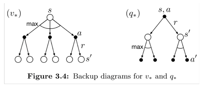
\[\begin{array}{l}{\text { 1. set } Q(s, a) \leftarrow r(s, a)+\gamma \mathbb{E}_{s^{\prime} \sim p\left(s^{\prime} | s, a\right)}\left[V\left(s^{\prime}\right)\right]} \\ {\text { 2. } \operatorname{set} V(s) \leftarrow \max _{a} Q(s, a)}\end{array}\]

Fitted Q-learning:

If the state space is high-dimensional or infinite, it is not feasible to represent $Q, V$ in a tabular form. In this case, we use two parameterized functions $Q_\phi, V_\phi$ to denote them. Then, we adopt fitted Q-iteration as stated in this paper:

\[\begin{array}{l}{\text { 1. set } y_{i} \leftarrow r\left(s_{i}, a_{i}\right)+\gamma \mathbb{E}_{s^{\prime} \sim p\left(s^{\prime} | s, a\right)}\left[V_{\phi}\left(s_{i}^{\prime}\right)\right]} \\ {\text { 2. } \operatorname{set} \phi \leftarrow \arg \min _{\phi} \sum_{i}\left\|Q_{\phi}\left(s_{i}, a_{i}\right)-y_{i}\right\|^{2}}\end{array}\]

Soft Policy Gradients

From the perspective of control as inference, we optimize for the following objective:

\begin{aligned} J(\theta) &= -D_{KL}(\hat{p}(\tau) || p(\tau)) \\ &= \sum_{t=1}^T \mathbb{E}_{(s_t, a_t) \sim \hat{p(s_t, a_t)}}[r(s_t, a_t)] + \mathbb{E}_{s_t \sim \hat{p}(s_t)}[\mathcal{H}(\pi(a_t|s_t))]\\ &= \sum_{t=1}^T \mathbb{E}_{(s_t, a_t) \sim p_\theta(s_t, a_t)}[r(s_t, a_t) - \log \pi(a_t|s_t)]\\ \end{aligned}

Now following the policy gradient method, such as REINFORCE, we just need to add a bonus entropy term to the rewards.

Soft Q-learning

Next, we connect the previous policy gradient to Q-learning. We can rewrite the policy gradient as follows:

Note that

\begin{aligned} \nabla_\theta \sum_{t=1}^T \mathbb{E}_{(s_t, a_t) \sim p_\theta(s_t, a_t)}[\log \pi(a_t|s_t)] &= \int \nabla_\theta \big[ p(\tau) \sum_{t=1}^T \log \pi(a_t|s_t)\big] d\tau\\ &= \int \nabla_\theta p(\tau)\sum_{t=1}^T \log \pi(a_t|s_t) + p(\tau) \nabla_\theta\sum_{t=1}^T \log \pi(a_t|s_t) d\tau\\ &= \int p(\tau) \nabla_\theta \log p(\tau)\sum_{t=1}^T \log \pi(a_t|s_t) + p(\tau) \nabla_\theta \log p(\tau) d\tau\\ &= \int p(\tau) \nabla_\theta \log p(\tau)\Big [ \sum_{t=1}^T \log \pi(a_t|s_t) + 1 \Big] d\tau.\\ \end{aligned}

Recall from the previous lecture, $\pi(a_t|s_t) = p(a_t | s_t, \mathcal{O}_{1:T}) = \exp(Q_\theta(s_t, a_t) - V_\theta(s_t))$

$V(s_t) = \log \int \exp(Q(s_t, a_t))da_t = \text{softmax}_{a_t} Q(s_t, a_t).$ Now combine these and rearrange the terms, we get:

\begin{aligned} \nabla_\theta J(\theta) &= \nabla_\theta \sum_{t=1}^T \mathbb{E}_{(s_t, a_t) \sim p_\theta(s_t, a_t)}[r(s_t, a_t) - \log \pi(a_t|s_t)]\\ &\approx \frac{1}{N}\sum_{i=1}^N\sum_{t=1}^T \nabla_\theta \log\pi_\theta(a_t|s_t) \Big[ r(s_t, a_t) + \big(\sum_{t'=t+1}^T r(s_{t'}, a_{t'}) - \log \pi_\theta(a_{t'}|s_{t'})\big) - \log \pi_\theta (a_t|s_t) - 1 \Big] \\ &= \frac{1}{N}\sum_{i=1}^N\sum_{t=1}^T \Big(\nabla_\theta Q_\theta(s_t, a_t) - \nabla_\theta V_\theta(s_t)\Big) \Big[ r(s_t, a_t) + Q_\theta(s_{t'}, a_{t'}) - Q_\theta(s_t, a_t) + V(s_t) \Big] \\ &\approx \frac{1}{N}\sum_{i=1}^N\sum_{t=1}^T \nabla_\theta Q_\theta(s_t, a_t) \Big[ r(s_t, a_t) + \text{soft} \max_{a_{t'}} Q_\theta(s_{t'}, a_{t'}) - Q_\theta(s_t, a_t) \Big] \\ \end{aligned}

Now the soft Q-learning update is very similar to Q-learning: $\theta \gets \theta + \alpha\nabla_\theta Q_\theta(s,a)(r(s,a) + \gamma V(s') - Q_\theta(s,a)),$ where $V(s') = \text{soft}\max_{a'} Q_\theta(s', a') = \log \int \exp (Q_\theta(s', a')) da'.$ Additionally, we can set the temperature in softmax to control the tradeoff between entropy and rewards.

To summaize, there are a few benefits of soft optimality:

Improve exploration and prevent entropy collapse
Easier to specialize (finetune) policies for more specific tasks
Principled approach to break ties
Better robustness (due to wider coverage of states)
Can reduce to hard optimality as reward magnitude increases