Lecture 23: Bayesian non-parametrics (continued)

Overview of inference in Dirichlet processes, topic models and the hierarchical Dirichlet process, and infinite latent variable models.

Recap

When using a mixture model, we need to answer the question: How many components (mixtures) to use? One method of answering this question is through Bayesian nonparametric mixture models: define a distribution over mixture models. Letting the number of mixture components go to infinity a priori equips the model with flexibility to match the number of components required by the data.

The infinite component prior can be achieved through a Dirichlet Process (DP). The DP can be intuitively defined through the Chinese Restaurant Process (CRP):

• Given a restaurant with an infinite number of tables (components) each with a potentially infinite number of seats (can account for unbounded number of data points).
• The first customer (data point) picks any table.
• The \(n\)th customer (data point) enters the restaurant and
  • Sits at an existing table (component) with probability \(\frac{m_{k}}{n-1+\alpha}\), where \(m_{k}\) is the number of people (data points) at table (component) \(k\).
  • Starts a new table (instantiates new component) with probability \(\frac{\alpha}{n-1+\alpha}\).

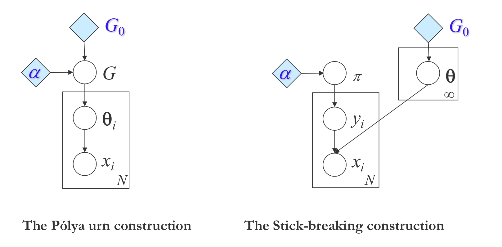
The DP can be equivalently defined through the stick-breaking process.

• Given a stick of length 1.
• For \(k=1,2,...\)
  • Sample \(b_{k} \sim \text{Beta}(1, \alpha)\).
  • Break of a fraction \(b_{k}\) of the stick. This corresponds to the size of the \(k\)th atom.
  • Sample a random location for this atom from some base distribution \(G_{0}\).
  • Recurse on the remaining stick.

We can define this sampling process as follows

\begin{aligned} G &= \sum_{k=1}^{\infty} \pi_{k} \delta_{\theta_{k}} \\ \theta_k &\sim G_{0} \\ \pi_{k} &= b_{k} \prod_{j=1}^{k-1}(1-b_{k}) \end{aligned}

Finally, we can also define the DP through the Pólya urn scheme:

• Suppose an urn contains \(\alpha\) black balls.
• For $n=1,2,…$, sample a ball from the urn at random.
  • If the ball is black, add a ball of a previously unseen color, along with the black ball, back into the urn.
  • If the ball is not black, add a new ball of the same color, along with the sampled ball, back into the urn.

Inference in the Dirichlet Process Gibbs Samplers, Dirichlet Process Notes

Given a Dirichlet process mixture model and a dataset that presumably has been generated from the model, inference is the process of determining the component of the mixture model from which each of the data point came from. Let us consider a Dirichlet process mixture model:

\[\begin{aligned} G := \sum_{k=1}^{\infty} \pi_{k} \delta_{\theta_{k}} & \sim \operatorname{DP}(\alpha, H) \\ \phi_{n} & \sim G \\ x_{n} & \sim f\left(\phi_{n}\right) \end{aligned}\]

where the data point $x_{n}$ is generated from the component $\phi_{n}$ of the mixture model $G$. We want to determine the component $\phi_{n}$ for each data point $x_{n}$.

Collapsed Gibbs Sampler

The collapsed Gibbs Sampler integrates out $G$ to get a Chinese restaurant process (CRP). Since, samples in a CRP are exchangeable, we can always rearrange the ordering of data points so that any sampled data point $x_{n}$ is the last one. Let, $z_{n}$ be the cluster allocation of the $x_{n}$ and $K$ be the total number of instantiated clusters, then the probability of $x_{n}$ belonging to the $k^{th}$ cluster is given by:

Note that, there is always a non-zero probability of the data point $x_{n}$ not being associated to any of the $K$ existing clusters and leads to the instantiation of a new cluster.

However, there are a few problems with this approach:

• Updating only one data point at a time makes the algorithm infeasible for large datasets.
• In the case of two true clusters getting merged into a single cluster in the beginning (possibly due to bad initialization), it is unlikely that a single data point will break out and form a different cluster.
• Getting to the true distribution involves going through low probability states and mixing can often be very slow.
• Integrating out parameter for new features is difficult if the likelihood is not conjugate and requires approximation of the integration.

Blocked Gibbs Sampler

In the Blocked Gibbs Sampler, we instantiate $G$ instead of integrating it out. Although $G$ is infinite-dimensional, we can simply approximate it with a truncated stick-breaking process:

\[\begin{aligned} G^{K} : &= \sum_{k=1}^{K} \pi_{k} \delta_{\theta_{k}} \\ \pi_{k} &=b_{k} \prod_{j=1}^{k-1}\left(1-b_{j}\right) \\ b_{k} & \sim \operatorname{Beta}(1, \alpha) \text { for } k=1, \ldots, K-1 \\ b_{K} &= 1 \end{aligned}\]

Now, for any $x_{n}$, its assocation probability to the $k^{th}$ cluster can be computed as:

\[p(z_{n}|\text{rest}) \propto \pi_{k} f(w_{n}|\theta_{k})\]

To estimate $\pi_{k}$ we follow the stick-breaking process which can also be thought of as a sequence of binary decisions. For example, we select $z_{n}=1$ with probability $b_{1}$. If $z_{n} \neq 1$, then we select $z_{n}=2$ with probability $b_{2}$ and so on. Formally,

\[b_{k} | \text{rest} \sim \operatorname{Beta} \left(1+m_{k},\alpha+\sum_{j=k+1}^{K} m_{j}\right)\]

Unlike the Collapsed Gibbs Sampler, where we instantiate a new cluster with some non-zero probability, here we fix the maximum number of clusters ($K$) in the beginning only. This fixed truncation introduces some error in the inference.

Slice Sampler

In the Slice Sampler, we introduce random truncation in place of pre-determined fixed truncation as in Blocked Gibbs Sampler. By marginalizing out this random truncation, we recover our original Dirichlet process.

We introduce a random variable $u_{n}$ for each data point. The indicator $z_{n}$ is then sampled as follows:

\[p\left(z_{n}=k | \mathrm{rest}\right)= I\left(\pi_{k}>u_{n}\right) f\left(x_{n} | \theta_{k}\right)\]

where, $I\left(\pi_{k}>u_{n}\right)$ is an indicator function which will select only a finite number of possible clusters those with $\pi_{k} > u_{n}$. The conditional distribution for $u_{n}$ is a uniform distribution with range $0$ to $\pi_{z_{n}}$:

\[u_{n} | rest \sim \operatorname{Uniform}[0, \pi_{z_{n}}]\]

Conditioned on $u_{n}$ and cluster indicator $z_{n}$, $\pi_{k}$ can be sampled according to the Blocked Gibbs Sampler.

Here, we only need to represent a finite number of components $K$ such that

\[1 - \sum_{k=1}^{K} \pi_{k} < min(u_{k})\]

Slice sampler preserves the structure of blocked sampling, albeit the blocks are different for different points. Since, we do not have to integrate out $G$, it is much faster than Collapsed Gibbs Sampler.

Hierarchical Dirichlet Process

Motivation: Topic Models

As introduced in previous lectures, a topic model is a hierarchical graphical model for document description. Under a topic model,

• Each document is a distribution over topics;
• Each topic is a distribution over words;
• Each document is an unordered collection of words (bag-of-words) sampled from the topics;
• The topics are shared among documents.

Latent Dirichlet Allocation (LDA) (Figure 1) is a particular kind of topic model where the distribution over topics and the distribution over words are both Dirichlet distributions. In LDA, the number of topics $K$ is specified in advance. This naturally leads to the non-trivial question of how to choose the correct number of topics. We have seen that Dirichlet process enables us to model a Gaussian mixture with an unbounded number of components. Can we apply the same idea here, replace the Dirichlet distribution over topics with a Dirichlet process, and get an LDA with unbounded number of topics?

Figure 1. Graphical representation of Latent Dirichlet Allocation

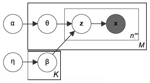
However, a naive implementation of Dirichlet process will fail in the case of topic models, because it cannot ensure the topics are shared. To be more specific, for a DP with a continuous base measure, we have zero probability of sampling the same atoms twice. As a result, a new set of topics will be generated every time we try to sample a document, making the topic model useless. Thus, we want the base measure to be discrete, but we don’t want to pin down the number of possible topics as in the original LDA. In other words, we need an infinite, discrete, random base measure, which leads to the Hierarchical Dirichlet Process (HDP) model proposed by Teh et al.

Hierarchical Dirichlet Process

The key observation of Teh et al. is that a sample from a Dirichlet process gives us exactly what we want – an infinite, discrete, random base measure. Hence, we can formulate a hierarchical Dirichlet process, where

\begin{aligned} G_0 \mid \gamma,H &\sim \mathrm{DP}(\gamma,H) \\ G_j \mid \alpha_0,G_0 &\sim \mathrm{DP}(\alpha_0,G_0) \end{aligned}

Here, $G_0$ is the global measure distributed as a Dirichlet process with concentration parameter $\gamma$ and base probability measure $H$. $G_j$ are the random measures which are conditionally independent given $G_0$, with distributions given by a Dirichlet process with base probability measure $G_0$. We can use $G_j$ to describe the distribution of topics for each document. Figure 2 shows a simple illustration of the sampling process of a HDP.

Figure 2. Sampling from a Hierarchical Dirichlet Process

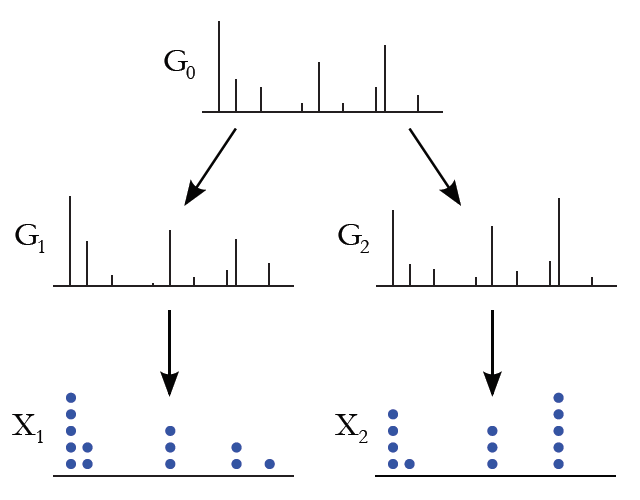
As in the case of DP, we can interpret HDP using the Chinese Restaurant Process analogy, where instead of a single restaurant, we now have a franchise of restaurants (documents). The restaurants share a common menu of dishes (topics). Each customer (word) picks a table in the restaurant and each table orders a dish (topic) according to the shared menu.

The following process desribes how to sample from a HDP-LDA. For more details, please refer to the paper .

• Sample the global measure $G_0\sim\mathrm{DP}(\gamma,H)$ (e.g. using stick breaking).
• For each document $j$
  • Sample a distribution over topics $G_j\sim\mathrm{DP}(\alpha_0,G_0)$.
  • For $i=1,\ldots,N_j$
    • Sample a topic $\phi_{ji}\sim G_j$.
    • Sample a word $w_{ji}\sim P(\phi_{ji})$.

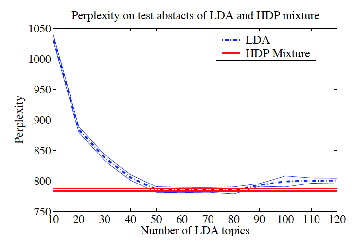
Figure 3 shows the perplexity score (i.e. negative log likelihood) of LDAs trained with different number of topics compared with HDP-LDA. It can be seen that HDP-LDA achieves the lowest possible perplexity by automatically selecting the “right” number of topics.

Figure 3. LDA vs. HDP-LDA

Latent Variable Models

Motivation

Latent class models introduced previously assume that classes are independent, which prevents the sharing of features across classes. However, in many applications it would be useful to share features across data points. For example,

• Images contain multiple objects which may have common features.
• Individuals in social networks may belong to multiple social groups.

Latent variable models introduce a latent feature space \(\mathbf{A}\), from which the data can be constructed. For example, in Factor Analyis, the data is assumed to be a linear combination of the features

\[\mathbf{X} = \mathbf{W} \mathbf{A}^T + \varepsilon\]

However, in general, it is not necessary for \(\mathbf{W}\) and \(\mathbf{A}\) to be combined linearly.

We are interested in answering the following two questions:

• Can we make the number of features (rows of \(\mathbf{A}\), columns of \(\mathbf{W}\)) unbounded?
• Can we do so in a manner that makes inference tractable?

We see that both of these properties can be achieved through the framework introduced by the Indian Buffet Process (IBP) Indian Buffet Process.

Sparse Latent Variable Models

We first consider the a large, but finite, sparse latent variable model. The sparsisty property is desirable so that as the number of features grows large, we can bound the expected number of non-zero features, which is a requirement for a tractable inference procedure.

The Chinese Restaurant Process discussed previously can be considered as a distribution over sparse finite bindary matrices, i.e. each customer (data point) is assigned to a single table (feature), leading to a matrix with a single non-zero entry per row.

Such a representation is excessively sparse, which motivates allowing multiple active features per row. In the restaurant analogy, this is equivalent to the customer sitting at multiple tables (or in IBP, get multiple dishes) - more on this later.

Let’s define our weight matrix as

\[\mathbf{W} = \mathbf{Z} \odot \mathbf{V}\]

where \(\mathbf{Z}\) is a sparse binary matrix.

We are interested in defining a distribution \(p(\mathbf{Z})\), which is achieved by placing a beta-Bernoulli prior over \(\mathbf{Z}\).

\[\pi_{k} \sim \text{Beta}\left(\frac{\alpha}{K}, 1\right), ~~ k=1,...,K\] \[z_{nk} \sim \text{Bernoulli}\left(\pi_{k}\right), ~~ n=1,...,N\]

Using the fact that the columns (features) of \(\mathbf{Z}\) are i.i.d. and the rows are i.i.d when conditioned on \(\pi_{k}\), and noting that the beta distribution is conjugate to the Bernoulli, the distribution over \(\mathbf{Z}\) is given by

\[p(\mathbf{Z}) = \prod_{k=1}^{K} \int \left(\prod_{n=1}^{N} p(z_{nk}| \pi_{k}) \right) p(\pi_{k}) d\pi_{k} = \prod_{k=1}^{K} \frac{\alpha}{K} \frac{\Gamma(m_k + \alpha/K) \Gamma(N - m_{k} + 1)} {\Gamma(N + 1 + \alpha/K)}\]

where \(m_{k} = \sum_{n=1}^{N} z_{nk}\) is the number of data points with active feature \(k\).

We can show that that this matrix is sparse by considering the expected number of non-zero entries

\[\mathbb{E}_{\pi_{1}, ..., \pi_{K}}\left[ \mathbf{1}^T \mathbf{Z} \mathbf{1} \right] = K \mathbb{E}_{\pi_{k}}\left[ \mathbf{1}^T \mathbf{z}_k \right] = K \sum_{n=1}^N \mathbb{E}_{\pi_{k}}\left[ z_{nk}\right] = K \sum_{n=1}^N \int_{0}^{1} \pi_{k} p(\pi_{k}) \mathrm{d} \pi_{k} = \frac{N \alpha}{1 + \frac{\alpha}{K}}\]

which is bounded above by \(N \alpha\).

Infinite Sparse Latent Variable Models

Taking \(K \rightarrow \infty\) in the model above would result in a matrices with infinite numbers of empty columns. To get arrow this, define an equivalence class \([\mathbf{Z}]\) of left-ordered binary matrices given by the function \(\mathit{lof}(\cdot)\). Specifically, the matrices are sorted in order of decreasing binary number defined by considering the rows of a single column as bits.

Binary matrix and the left ordered form. Taken from Indian Buffet Process.

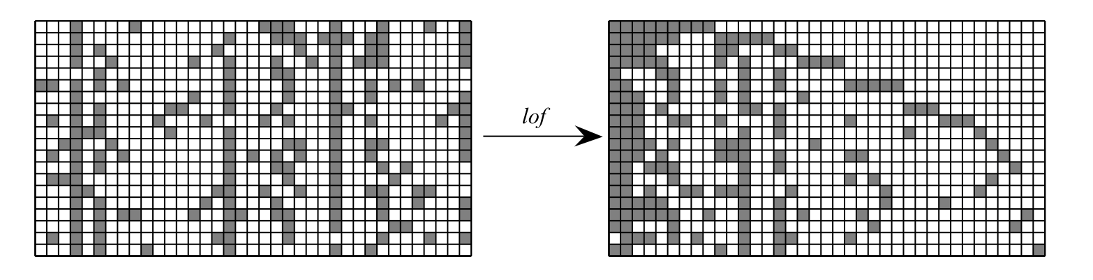
All matrices with the equivalence class \([\mathbf{Z}]\) have equal probability. The total probability of the class is then equal to \(| [\mathbf{Z} ] | p(\mathbf{Z})\), where \(| [\mathbf{Z} ] |\) is the number of matrices in the class. In order to compute \(| [\mathbf{Z} ] |\), we introduce a few terms

• Let the history of a feature $k$ be defined by the binary number equivalent of its rows, e.g. a 4 data point example with column \((0, 1, 0, 1)\) has history 5.
• Let $K_{h}$ denote the number of features with history $h$.
• Let $K_{+}$ denote the number of features with non-zero history.
• Let $K = K_{0} + K_{+}$, i.e. the sum of the zero history and non-zero history features.

For $N$ data points, we have a maximum history of $2^{N-1}$ (max N-bit binary number). Since columns are exchangeable, we note that any permutation of columns with history $h$ does not chage the matrix under \(\mathit{lof}\) equivalence.

\[| [\mathbf{Z} ] | = {K \choose {K_{0}...K_{2^{N}-1}}} = \frac{K!}{\prod_{h=0}^{2^{N}-1}K_h!}\]

The distribution over \([\mathbf{Z}]\) is then

\[p([\mathbf{Z}]) = |[\mathbf{Z}]|p(\mathbf{Z}) = \frac{K!}{\prod_{h=0}^{2^{N}-1}K_h!} \prod_{k=1}^{K} \frac{\alpha}{K} \frac{\Gamma(m_k + \alpha/K) \Gamma(N - m_{k} + 1)} {\Gamma(N + 1 + \alpha/K)}\]

We can evaluate this term by splitting \(K\) into the terms for which \(m_{k} = 0\) and \(m_{k} > 0\) (see eqn (13) in Indian Buffet Process)

\begin{aligned} p([\mathbf{Z}]) &= \left(\frac{\frac{\alpha}{K} \Gamma\left(\frac{\alpha}{K}\right) \Gamma(N+1)} {\Gamma\left(N+1+\frac{\alpha}{K}\right)}\right)^{K-K_{+}} \quad \prod_{k=1}^{K_{+}} \frac{\frac{\alpha}{K} \Gamma\left(m_{k}+\frac{\alpha}{K}\right) \Gamma\left(N-m_{k}+1\right)} {\Gamma\left(N+1+\frac{\alpha}{K}\right)} \\ &= \left(\frac{\frac{\alpha}{K} \Gamma\left(\frac{\alpha}{K}\right) \Gamma(N+1)} {\Gamma\left(N+1+\frac{\alpha}{K}\right)}\right)^{K} \quad \prod_{k=1}^{K_{+}} \frac{\Gamma\left(m_{k}+\frac{\alpha}{K}\right) \Gamma\left(N-m_{k}+1\right)} {\Gamma\left(\frac{\alpha}{K}\right) \Gamma(N+1)} \\ &= \left(\frac{N !}{\prod_{j=1}^{N}\left(j+\frac{\alpha}{K}\right)}\right)^{K} \quad \left(\frac{\alpha}{K}\right)^{K_{+}} \prod_{k=1}^{K_{+}} \frac{\left(N-m_{k}\right) ! \prod_{j=1}^{m_{k}-1}\left(j+\frac{\alpha}{K}\right)}{N!} \end{aligned}

Taking the limit as \(K \rightarrow \infty\)

\begin{aligned} \lim_{K \rightarrow \infty} p([\mathbf{Z}]) &= \lim_{K \rightarrow \infty} \frac{\alpha^{K_{+}}}{\prod_{h=1}^{2^{N}-1} K_{h} !} \cdot \frac{K !}{K_{0} ! K^{K_{+}}} \cdot\left(\frac{N!}{\Pi_{j=1}^{N}\left(j+\frac{\alpha}{K}\right)}\right)^{K} \cdot \prod_{k=1}^{K_{+}} \frac{\left(N-m_{k}\right) ! \Pi_{j=1}^{m_{k}-1}\left(j+\frac{\alpha}{K}\right)}{N !} \\ &= \quad \quad \frac{\alpha^{K_{+}}}{\prod_{h=1}^{2^{N}-1} K_{h} !} \cdot \quad \quad 1 \quad \quad \cdot \quad \exp \left\{-\alpha H_{N}\right\} \quad \cdot \prod_{k=1}^{K_{+}} \frac{\left(N-m_{k}\right) !\left(m_{k}-1\right) !}{N !} \end{aligned}

where \(H_{N} = \sum_{j=1}^{N} \frac{1}{j}\) is the $N$th harmonic number. See Appendix A in for more details about this limit.

Intuition: Indian Buffet Process

Setup: Buffet with infinite number of dishes. Customers can select any number of dishes.

Procedure:

• Customer enters restaurant and selects \(\text{Poisson}(\alpha)\) dishes.
• The \(n\)th customer considers each previously selected dish and selects from it with probability \(\frac{m_{k}}{n}\).
• The \(n\)th customer then selects \(\text{Poisson}(\frac{\alpha}{n})\) new dishes.

We can show that this sequential process is lof-equivalent to the infinite beta-Bernoulli model defined previously.

\begin{aligned} p(\mathbf{Z}) &= \prod^{N}_{n=1} p\left(\mathbf{z}_{n} | \mathbf{z}_{1 :(n-1)}\right) \\ &=\prod_{n=1}^{N} \operatorname{Poisson}\left(K_{1}^{(n)} | \frac{\alpha}{n}\right) \prod_{k=1}^{K_{+}}\left(\frac{\sum_{i=1}^{n-1} z_{i k}}{n}\right)^{z_{n k}} \left(\frac{n-\sum_{i=1}^{n-1} z_{i k}}{n}\right)^{1-z_{n k}} \\ &=\prod_{n=1}^{N}\left(\frac{\alpha}{n}\right)^{K_{1}^{(n)}} \frac{1}{K_{1}^{(n)} !} e^{-\alpha / n} \prod_{k=1}^{K_{+}}\left(\frac{\sum_{i=1}^{n-1} z_{i k}}{n}\right)^{z_{n k}} \left(\frac{n-\sum_{i=1}^{n-1} z_{i k}}{n}\right)^{1-z_{n k}}\\ &=\frac{\alpha^{K_{+}}}{\prod_{n=1}^{N} K_{1}^{(n)} !} \exp \left\{-\alpha H_{N}\right\} \prod_{k=1}^{K_{+}} \frac{ ( N-m_{k} ) !\left(m_{k}-1\right) !}{N !} \end{aligned}

where \(K_{1}^{(n)}\) is the number of new features in the \(n\)th row. Accounting for the cardinality of the lof-equivalence set gives the same result as the beta-Bernoulli case.

Summary

The IBP enables reasoning about a potentially infinite number of features, which can be selected in a data-dependent manner. The capacity of the model (in terms of # of features) does not need to be specified a priori, but can be controlled through a prior distribution over the feature selection matrices. Some properties of the IBP

• “Rich get richer” - popular dishes (features selected by many data points) become more popular (are assigned to more data).
• The number of dishes selected by a customer (non-zero entries in each data row) is distributed according to \(\text{Poisson}(\alpha)\).
• The number of dishes selected by all customers (number of non-zero entries) is distributed according to \(\text{Poisson}(N \alpha)\).
• The number of dishes selected by any customer (number of non-zero columns) is distributed according to \(\text{Poisson}(\alpha H_{n})\).
• The total number of dishes selected (number of non-zero entries) in expectation is bounded by \(N \alpha\).