Lecture 24: Integrative Paradigms of GM: Regularized Bayesian Methods

Regularized Bayesian Methods and some applications.

Learning GMs

There are different frameworks to learn GMs: First, Bayesian framework. It allows priors to be introduced. Both parametric and nonparametric Bayesian tricks can be applied to learning these models. Second, max-margin framework. SVM is an example of this framework(it can be used to learn not only a classifier but also a graphical model). Third, there are also the kernel methods, of which SVM is also an example. Gaussian processes, another nonparametric bayesian paradigm, is another example of application of kernel methods.

These frameworks has complementary advantages of one another. For example, in the Bayesian framework, we have prior knowledges, we can bypass model selection; in SVM, outliers do not affect the results, etc. It is possible to use the ideas of these different frameworks and enjoy the advantages of all in one single paradigm. Potentially these ideas could be used to further empower the already powerful deep-learning models, which would be an interesting new topic to explore in the future.

Bayesian inference

We are already familiar with the Bayes’ rule: $p(\mathcal{M}\vert x) = \frac{p(x\vert\mathcal{M})\pi(\mathcal{M})}{\int p(x\vert\mathcal{M})\pi(\mathcal{M})d\mathcal{M}}$ where $\mathcal{M}$ is a model from some hypothesis space, $x$ is observed data. The Bayesian framework allows you to derive a posterior distribution of the model. The prior distribution, i.e. the $\pi(\mathcal{M})$ part of the model needs to be provided, usually selected by the needs, while the $p(\mathbf{x}\vert\mathcal{M})$ part of the model need to be designed and could be the graphical part.

In parametric Bayesian inference, $\mathcal{M}$ is represented as a finite set of parameters $\theta$.

a parametric likelihood: $\mathbf{x} \sim p(\cdot\vert\theta)$
Prior on $\theta$: $\pi(\theta)$
Posterior: $p(\theta \vert \mathbf{x}) = \frac{p(\mathbf{x}\vert\theta)\pi(\theta)}{\int p(\mathbf{x}\vert\theta)\pi(\theta)d{\theta}} \propto p(\mathbf{x}\vert\theta)\pi(\theta)$

You don’t make too much flexibility in the choice of the model itself. You can make a choice of a Gaussian model or a Dirichlet distribution, the flexibility is in the way how it is parameterized. Define a prior distribution of the parameters, and you’ll get a posterior distribution of the parameters.

In nonparametric Bayesian inference, $\mathcal{M}$ is a richer model.

Nonparametric likelihood: $\mathbf{x} \sim p(\cdot\vert\mathcal{M})$
Prior on $\mathcal{M}$: $\pi(\mathcal{M})$
Posterior: $ p(\mathcal{M}\vert x) = \frac{p(x\vert\mathcal{M})\pi(\mathcal{M})}{\int p(x\vert\mathcal{M})\pi(\mathcal{M})d\mathcal{M}} \propto p(x\vert\mathcal{M})\pi(\mathcal{M})$

The model itself becomes a space for you to make inference on. For example you have an unknown number of components in a mixed model, or an unknown number of dimensions in the latent feature models. Popular nonparametric Bayesian models include Dirichlet Process, Indian Buffet process and Gaussian process. These models are more powerful than the parametric Bayesian models. Nonparametric Bayesian models allow us to pay more attention to the power of data, and the interplay between the data and prior is more natural. It allows us to bypass the model selection problem and let the data itself determine model complexity.

There is a new, different expression of Bayes’ rule (Zellner, Am. Stat. 1988):

$\min_{p(\mathcal{M})} \text{KL}(p(\mathcal{M})\Vert \pi(\mathcal{M})) - \mathbb{E}_{p(\mathcal{M})}[log(p(x\vert\mathcal{M}))]$

$\text{s.t.}: p(\mathcal{M})\in\mathcal{P}_{\text{prob}}$

$\mathcal{P}_{\text{prob}}$ is a direct but trivial constraint on the posterior distribution. This variation of expression of Bayes’ rule turns the problem into a optimization problem. It also gives space to inference algorithms, or even to augment the model. This new expression can be used to steer the Bayes inference into some interesting directions.

With this expression we can play some tricks in redefining the space of the posterior distribution. The trivial constraint $\mathcal{P}_{\text{prob}}$ that guarantees whatever distributions are allowed can also be tightened to ensure that only a subset of distributions are allowed. The subset can be defined due to constraint from data. For example: $\inf_{q(\mathcal{M}),\xi}\text{KL}(q(\mathcal{M})\Vert\pi(\mathcal{M})) -\int_{\mathcal{M}}\log p(\mathcal{D}\vert\mathcal{M})q(\mathcal{M})d\mathcal{M} + U(\xi)$ $\text{s.t.:}q(\mathcal{M})\in\mathcal{P}_\text{post}(\xi)$ where, e.x.,

$\mathcal{P}_\text{post}(\xi) \overset{\mathrm{def}}{=} \Big\{q(M)\vert\forall t=1,\dots, T, h(Eq(\psi_t; \mathcal{D}))\leq\xi_t\Big\},$

and $U(\xi) = \sum_{t=1}^{T}\mathbb{I}(\xi_t=\gamma_t)=\mathbb{I}(\xi=\gamma).$

For every data points you can constrain the distribution to satisfy the margin, and that gives you a new set of posterior distributions.

MLE versus Max-margin learning

Now let’s put MLE and Max-margin learning side by side for comparison. For likelihood-based classification, a typical example is logistic regression. And for Max-margin learning, the example would be SVM.

In the classical predictive models the input and output spaces are $\mathcal{X}\triangleq\mathbb{R}^{M_x}\quad \mathcal{Y}\triangleq\{-1,+1\}.$ We are learning $\mathbb{w} = \text{arg}\min_{\mathbf{w}\in\mathcal{W}}\ell(x,y;\mathbf{w}+\lambda R(\mathbf{w}))$ where $\ell(\cdot)$ represents a convex loss, and $R(\mathbf{w})$ is a regularizer to prevent overfitting.

In logistic regression, the maximum likelihood estimation is $\max_{\mathbf{w}}\mathcal{L}(\mathcal{D}; \mathbf{w}) \triangleq \sum_{i=1}^{N}\log p(y^i \vert x^i; \mathbf{w}) + \mathcal{N}(\mathbf{w})$ i.e. you are maximizing the likelihood of the label given the data points. A regularizer $\mathcal{N}(\mathbf{w})$ could be introduced. This is sometimes called a shrinkage function.

It corresponds to a log loss with L2R:

\[\ell_{LL}(x,y;\mathbf{w}) \triangleq \ln \sum_{y'\in\mathcal{Y}} \exp \{ \mathbf{w}^\top\mathbf{f}(x, y')\} -\mathbf{w}^\top\mathbf{f}(x, y)\]

SVM is formulated very differently:

$\min_{\mathbf{w},\xi}\frac{1}{2}\mathbf{w}^\top\mathbf{w} + C\sum_{i=1}^{N}\xi_i; \quad$ $\text{s.t.} \forall{i},\forall{y'\neq y}:\mathbf{w}^\top\Delta\mathbf{f}_i(y')\geq1-\xi_i,\, \xi_i\geq 0.$

It corresponds to a hinge loss with L2R:

\[\ell_{MM}(x,y;\mathbf{w}) \triangleq \max_{y' \in \mathcal{Y}}\mathbf{w}^\top\mathbf{f}(x,y') - \mathbf{w}^\top\mathbf{f}(x,y) + \ell'(y', y)\]

The two learning paradigms have complementary advantages. Likelihood-based models are probablistic, therefore by introducing a prior distribution, Bayesian learning can be easily performed. Besides, probablistic models allow for introduction of latent variables so that you can have enable latent space models. SVM, on the other hand, does not allow for hidden variables because it is non-probablistic. But the advantages are that the support vector property gives good guarantee on generizability, and that it allows for kernel tricks.

The Maximum Entropy Discrimination (MED) is an approach to combine the logistic regression and SVM. Model averaging $y = \text{sign} \int p(\mathbf{w})F(x;\mathbf{w}), (y\in\{+1, -1\})$ The optimization problem (binary classification) is:

\[\min_{p(\Theta)} \text{KL}(p(\Theta)\Vert p_0(\Theta))\] \[\text{s.t.}\quad\int p(\Theta)\big[y_iF(x;\mathbf{w}-\xi_i)\big]d\Theta\geq0, \forall{i},\]

where $\Theta$ is the parameter $\mathbf{w}$ when $\xi$ are kept fixed or the pair $\mathbf{w},\xi$ when we want to optimize over $\xi$. This is a mechanical combination of the two approaches because the margin idea is used to define constraints to the posterior, and the likelihood idea to define the loss.

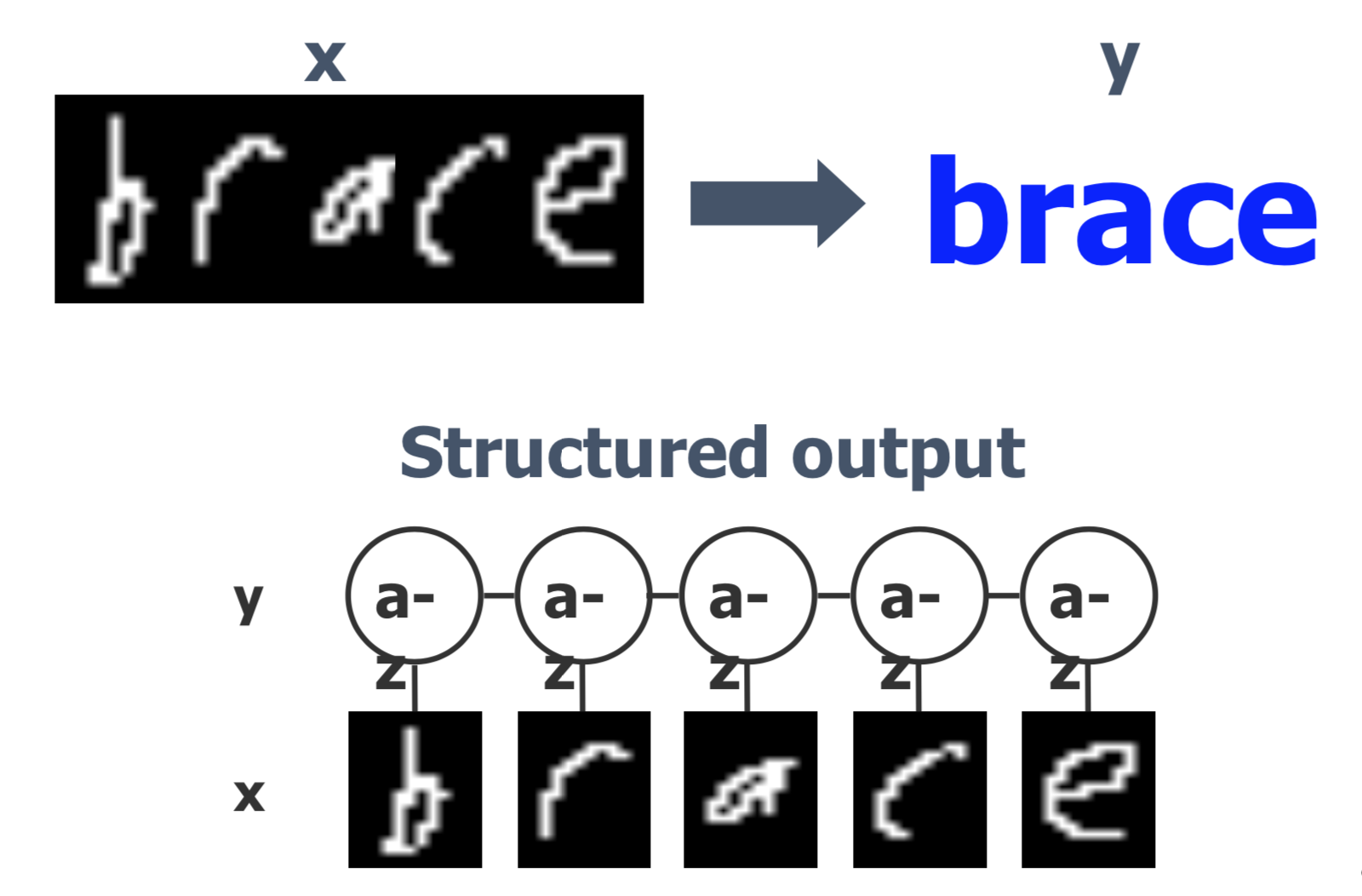
Structured Prediction Graphical Models

Conditional Random Fields (CRF) is based on a logistic loss. It could be seen as a structured version of logistic regression with the input and output spaces $\mathcal{X}\triangleq\mathbb{R}_{X_1}\times,\dots,{R}_{X_K} , \mathcal{Y}\triangleq \mathcal{R}_{Y_1}\times,\dots,{R}_{Y_K}$.

The max-likelihood estimation (point-estimate) is: $\mathcal{L}(\mathcal{D};\mathbf{w}) \triangleq \log \sum_{y'}\exp{(\mathbf{w}^\top\mathbf{f}(x,y'))}-\mathbf{w}^\top\mathbf{f}(x,y) + R(\mathbf{w})$

Max-Margin Markov Networks are based on a hinge loss. It is a structured version of SVM with the input and output spaces $\mathcal{X}\triangleq\mathbb{R}_{X_1}\times,\dots,{R}_{X_K} , \mathcal{Y}\triangleq \mathcal{R}_{Y_1}\times,\dots,{R}_{Y_K}$.

The max-margin learning (point-estimate): $\mathcal{L}(\mathcal{D};\mathbf{w})\triangleq \log\max_{y'}\mathbf{w}^\top\mathbf{f}(x,y') - \mathbf{w}^\top\mathbf{f}(x,y) + \ell(y',y) + R(\mathbf{w})$

We have seen some examples of how models can be generalized, now we will see how to combine them. If we change the boundary of SVM to a family of boundaries, we get MED; if we make SVM structured and make multi-labeled, coupled prediction, M$^3$N is what we get. Naturally, the next thing we can do is to combine the two and can have a distribution of the structured SVM as well. And thus we get the maximum entropy discrimination Markov networks (MED-MN).

Maximum Entropy Discrimination Markov Networks

Structured MaxEnt Discrimination (SMED):

\begin{aligned} \min _{p(w), \xi} \operatorname{KL}(p(w) \| p_0(w))+U(\xi)\\ \text { s.t. } : p(w) \in \mathcal{F}_1,\xi\geq 0,\forall i \end{aligned}

This is also know as generalized maximum entropy or regularized KL-divergence.

Feasible subspace of weight distribution:

\begin{aligned} \mathcal{F}_1 = \{p(w):\int p(w)[\Delta F_i(y;w)-\Delta l_i(y)]dw\geq -\xi_i,\forall i, \forall y \neq y^i\} \end{aligned}

Average from distribution of $M^3Ns$:

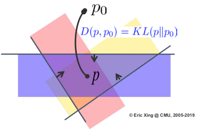
\begin{aligned} h_1(x;p(w)) = \arg \max_{y\in \mathcal{Y}(x)}\int p(w)F(x,y;w)dw \end{aligned}

We are going to use a loss function which consists of the KL divergence between the posterior distribution and the prior distribution, plus a slack function to capture the margin error like in SVM. The posterior distribution is constrained to the function space known as predictive margin for every data point. This optimization procedure also includes a predictive rule, which uses the model averaging idea that integrates over all the values of the weights and gets an ensemble prediction.

This formulation is different from pure maximum margin learning or pure maximum likelihood learning. KL divergence is a mapping the distances between distributions. And we are doing distribution learning in a constrained space, which is represented by the colored areas. Essentially our final goal is to project the constrained space into the KL divergence.

Solution to MaxEnDNet

Posterior Distribution: $p(w) = \frac{1}{Z(\alpha)}p_0(w)\exp \{\sum_{i,y}\alpha_i(y)[\Delta F_i(y,w)-\Delta l_i(y)]\}$

Dual Optimization Problem:

\begin{aligned} D1: \max_\alpha -\log Z(\alpha) -U^*(\alpha)\\ \text { s.t. } : \alpha_i(y)\geq 0,\forall i, \forall y,\\ \end{aligned}

The derived posterior distribution is similar to a Bayes law. The key idea behind the SVM derivation is that there is a primal dual conversion in the optimization where you are turning the problem of solving for the decision boundary weight into a problem where you solve for alphas. The index of the decision boundary weight spans over the dimension, while the index the alphas spans over the number of data. Due to the complementary slackness constraint, we know alpha is zero for most data points because they are not on the decision boundaries.

This is very interesting as we are essentially doing Bayesian inference which incorporates the prior. At the same time we also achieve the support vector effect by estimating the dual parameters, which only depend on a few data points in the training set. This is one fo the key advantages of SVM. The solution to MaxEnDNet is able to merit these two things together. However, solving the MaxEnDNet problem is not necessarily a easy problem depending on the prior. If the prior is Gaussian, then the whole formulation is reduced to a structural SVM.

Algorithmic issues of solving $M^3Ns$:

Formulation of the primal problem:

\begin{aligned} P0(M^3N):\min \frac{1}{2}||w||^2&+C\sum_{i=1}^N\xi_i\\ \text { s.t. }\forall i,\forall y\neq y^i:w^T\Delta f_i(y)&\geq \Delta l_i(y)-\xi_i,\\ \xi_i\geq 0 \end{aligned}

Algorithms used to solve the primal problem: Cutting Plane, Sub Gradient, etc.

Formulation of the dual problem:

\begin{aligned} D0(M^3N): \max_\alpha \sum_{i,y}\alpha_i(y)\Delta l_i(y) &-\frac{1}{2}\eta^T\eta\\ \text{ s.t. }\forall i,\forall y: \sum_{y}\alpha_i(y)&=C;\alpha_i(y)\geq 0,\\ \text{where } \eta &= \sum_{i,y}\alpha_i(y)\Delta f_i(y) \end{aligned}

Algorithms used to solve the dual problem: SMO, Exponentiated Gradient etc.

Variational Learning of LapMEDN

Exact primal or dual function is hard to optimize.

Primal form: $\min_{\mu,\xi}\sum_{k=1}^K(\sqrt{\mu_k^2+\frac{1}{\lambda}}-\frac{1}{\sqrt{\lambda}}\log \frac{\sqrt{\lambda \mu_k^2+1}+1}{2})+C\sum_{i=1}^N\xi_i$

With the following constraint: $\mu^T\Delta f_i(y)\geq \Delta l_i(y)-\xi_i,\xi_i\geq 0,\forall i,\forall y \neq y^i$

Dual form:

\begin{aligned} \max_\alpha \sum_{i,y}\alpha_i(y)\Delta l_i(y) - \sum_{k=1}^K\log \frac{\lambda}{\lambda - \eta_k^2}\\ \text{ s.t. } \sum_{y}\alpha_i(y) = C;\alpha_i(y)\geq 0, \forall i, \forall y \end{aligned}

Instead, we can use the hierarchical representation of Laplace prior and get the following:

\begin{aligned} KL(p||p_0) \leq -H(p)-<\int q(\tau)\log \frac{p(w|\tau)p(\tau|\lambda)}{q(\tau)}d\tau>_p =L(p(w),q(\tau)) \end{aligned}

Then we can optimize this derived upper bound: $\min_{p(w)\in F_1;q(\tau);\xi}L(p(w),q(\tau))+U(\xi)$

The advantages of MEDN

An averaging Model: PAC-Bayesian prediction error guarantee. It gives practitioners insight about how to reduce the complexity and training costs.
Entropy regularization: Introducing useful biases. The bayesian framework allows you to control the sparsity and behavior of the weight in a soft way. What is achieved by the PAC-based model is that it gives a range of constraints like the L1/L2 constaints, depending on how you adjust the hyper-parameters in the laplace prior in the MaxEnDNet. You will have a smooth middle ground among L1, L2 and other constraints.
Integrating Generative and Discriminative principles
Incorporate latent variables and structures. Latent variable is rarely explored formally in a SVM framework, but very often in a bayesian framework. Allowing latent variables in this bayesian SVM brings out interesting result.

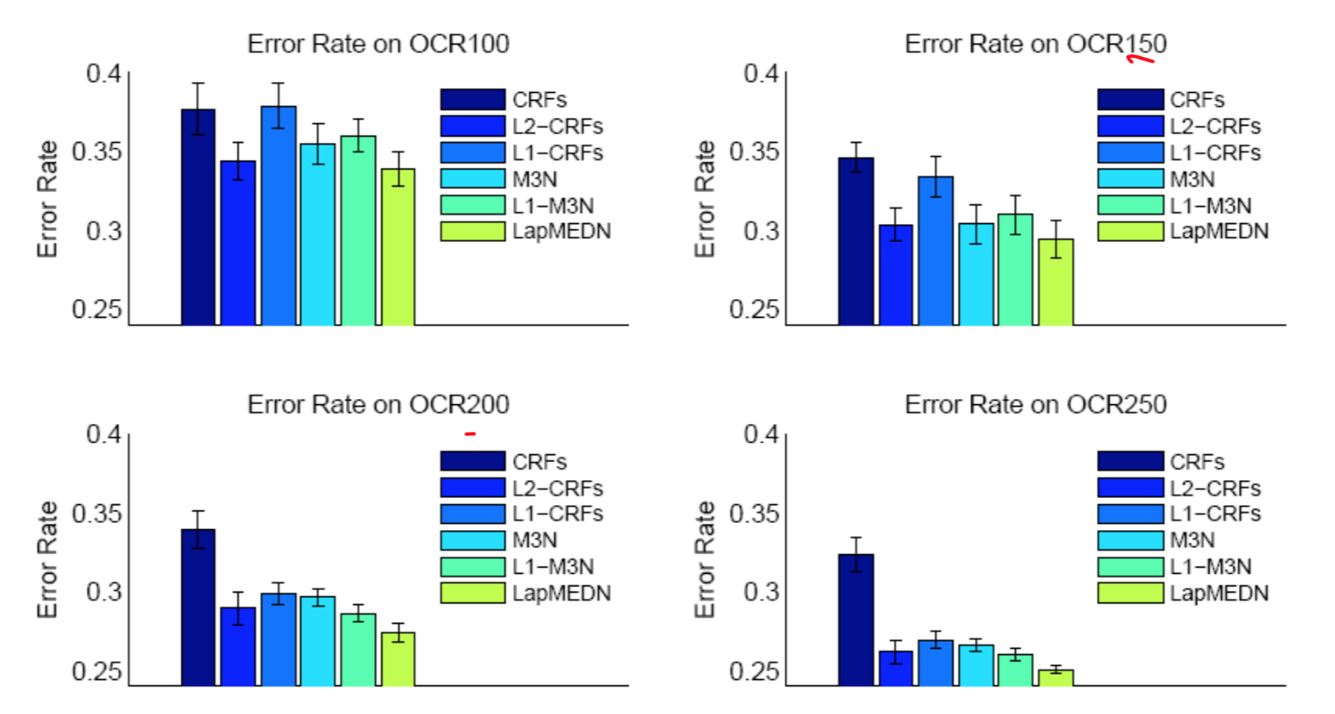
Experimental results on OCR datasets

Regardless of the size of training data, the LapMEDN model consistently outperforms the other models.

Structural output example for ambiguous image

Compare LapMEDN with baselines under situations with different amount of data

Partially Observed MaxEnDNet (PoMEN)

PoMEN learning:

\[\min_{p(w,\{z\}),\xi}KL(p(w,\{z\})||p_0(w,\{z\}))+U(\xi)\]

With the following specification:

\[p(w,(z))\in \mathcal{F}_2,\xi_i \geq 0,\forall i\]

And:

\[\mathcal{F}_2=\{p(w,z)\}: \sum_z\int p(w,z)[\Delta F_i(y,z;w)-\Delta l_i(y)]dw\geq -\xi_i,\forall i, \forall y\neq y^i\]

Prediction:

\[h_2(x)=\arg \max_{y\in \mathcal{Y}(x)}\sum_z\int p(w,z)F(x,y,z;w)dw\]

Above can be optimized using alternating minimization algorithm.

Step 1: keep $p(z)$ fixed, optimize over $p(w)$.

Step 2: keep $p(w)$ fixed, optimize over $p(z)$.

Predictive Latent Subspace Learning via a large-margin approach

There are some latent space models, such as Latent Dirichlet Allocation(LDA)， Principal Component Analysis(PCA). One of major utility of latent space models is to get embeddings. Most of time, we want to use the embeddings to make better predictions. Finding latent subspace representations is an old topic, which means mapping a high-dimensional representation into a latent low-dimensional representation, where each dimension can have some interpretable meaning.

In the past, the whole process can be divided into two steps. Firstly, get the embedded features of every text. Secondly, use the embedded feature as augmented data to retrain a classifier. The classification error, which can be represented as a loss function, is different from the embedding loss function. But now, we try to coalesce the two steps, which can be called as predictive subspace learning with supervision.

Unsupervised latent subspace representations are generic but can be sub-optimal for predictions. Many datasets are available with supervised side information. They can be noisy, but not random noise. For example, labels and rating scores are usually assigned based on some intrinsic property of the data. So it is helpful to suppress noise and capture the most useful aspects of the data. The final goal is to discover latent subspace representations that are both predictive and interpretable by exploring weak supervision information.

LDA: Latent Dirichlet Allocation

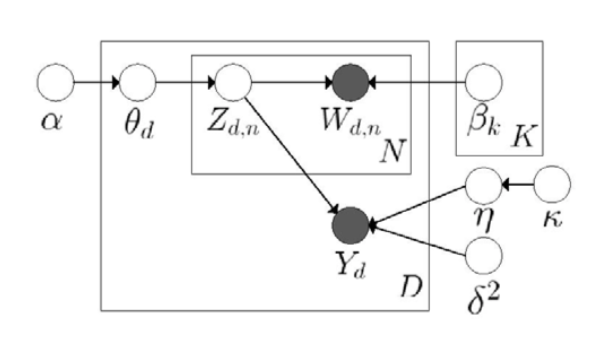
As shown below, the model tries to get latent variables for every word. During the process, it needs to initialize the Dirichlet parameter, and get the latent topic vector for every documents. The generative procudure is

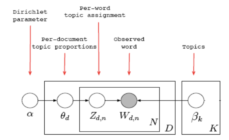
Generative Procedure:

For each document $d$:

Sample a topic proportion $\theta_{d} \sim Dir(\alpha)$

For each word:

Sample a topic $Z_{d,n} \sim Mult(\theta_{d})$

Sample a word $W_{d,n} \sim Mult(\beta_{z_{d,n}})$

The joint distribution is

\[p(\theta, \mathbf{z}, \mathbf{W} | \alpha, \beta)=\prod_{d=1}^{D} p\left(\theta_{d} | \alpha\right)\left(\prod_{n=1}^{N} p\left(z_{d n} | \theta_{d}\right) p\left(w_{d n} | z_{d n}, \beta\right)\right)\]

But exact inference is intractable, and variational inference is

\[q(\mathbf{z}, \theta) \sim p(\mathbf{z}, \theta | \mathbf{W}, \alpha, \beta)\\ \mathcal{L}(q) \triangleq-E_{q}[\log p(\theta, \mathbf{z}, \mathbf{W} | \alpha, \beta)]-\mathcal{H}(q(\mathbf{z}, \theta)) \geq-\log p(\mathbf{W} | \alpha, \beta)\]

In this way, we can minimize the variational bound to estimate parameters and infer the posterior distribution.

Maximum Entropy Discrimination LDA(MedLDA)

Use the latent representations $Z_{d,n}$ to make a prediction of the label. So that the training of LDA becomes a supervised training. And the goal is to influence $\theta$ indirectly, and let embeddings to be more oriented, to be more discriminative.

MED estimation can be divided into MedLDA regression model and MedLDA classification model. In MedLDA models, they replace the likelihood function by Bayesians LDA to make it a LDA based loss function. And then plus the prediction penalty on the margin, and constrain these margins. This can be pretty flexible, since it has two types of LDA. For example, predicting the score of the service based on the latent variables of the Yelp comments can use MedLDA Regression Model, and when predicting the label, it can use MedLDA Classification Model. The objective function considers predictive accuracy and model fitting. So it augments the original LDA by adding some new components.

The objective function and constraints for MedLDA Regression Model is

\[P_{1}(MedLDA^{r}): \min_{q, \alpha, \beta, \delta^{2}, \xi, \xi^{*}} \mathcal{L}(q)+C \sum_{d=1}^{D}\left(\xi_{d}+\xi_{d}^{*}\right)\\ \text {s.t. } \forall d : \left\{\begin{array}{ll}{y_{d}-E\left[\eta^{T} \overline{Z}_{d}\right] \leq \epsilon-\xi_{d},} & {\mu_{d}} \\ {-y_{d}-E\left[\eta^{T} \overline{Z}_{d}\right] \leq \epsilon+\xi_{d}^{*},} & {\mu_{d}^{*}} \\ {\xi_{d} \geq 0,} & {v_{d}} \\ {\xi_{d}^{*} \geq 0,} & {v_{d}^{*}}\end{array}\right.\]

The objective function and constraints for MedLDA Classification Model is

\[\mathrm{P} 2\left(\operatorname{MedLDA}^{c}\right) : \min _{q, q(\eta), \alpha, \beta, \xi} \mathcal{L}(q)+C \sum_{d=1}^{D} \xi_{d}\\ \text { s.t. } \forall d, y \neq y_{d} : \quad E\left[\eta^{\top} \Delta \mathbf{f}_{d}(y)\right] \geq 1-\xi_{d} ; \xi_{d} \geq 0\]

Comparision between LDA and supervised LDA

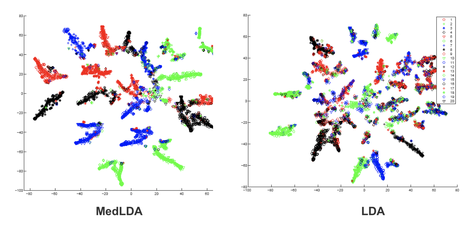
The embedding performance of original LDA and supervised LDA can be seen from Figure in the experiment of document modeling. The embeddings of original LDA are less discrimitive, which is shown that different colors overlap with each other. But embeddings from supervised LDA are more separatly. Therefore, MedLDA makes the classification problem easier.

Classification

In classification problems, the baseline is LDA + SVM, which has two separate steps. Models of sLDA and DiscLDA are probabilistic supervised topic models, and models of MedLDA and MedLDA + SVM are maximum margin based SVM models. And the models based on maximum margin principle perform best. The measurement is relative improvement ratio.

\[R R(\mathcal{M})=\frac{\text { precision }(\mathcal{M})}{\text {precision}(L D A+S V M)}-1\]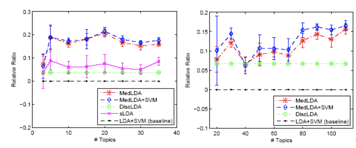

Regression

The performance of regression is same as classification. The combination of likelihood and margin based procedure has the best performance. The measurement is predictive $R^{2}$ and per-word log-likelihood.

\[p R^{2}=1-\frac{\sum_{d}(y_{d}-\hat{y}_{d})^{2}}{\sum_{d}(y_{d}-\bar{y_{d}})^{2}}\]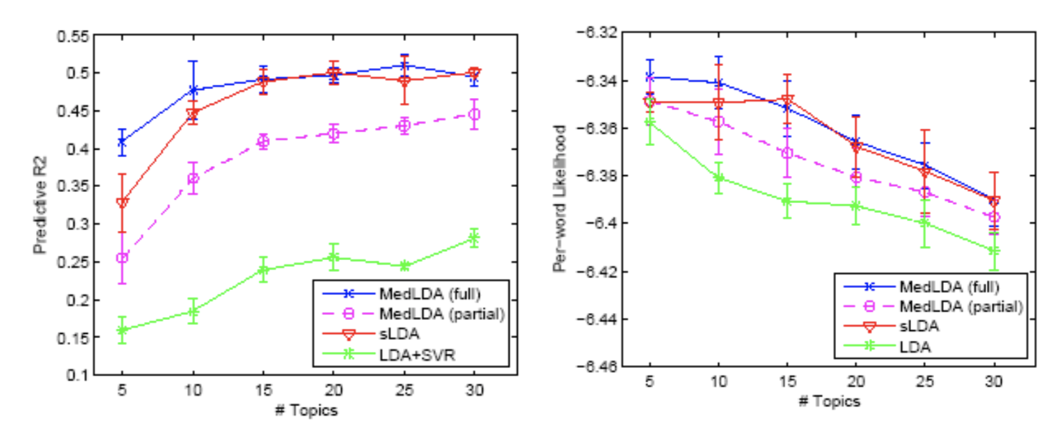

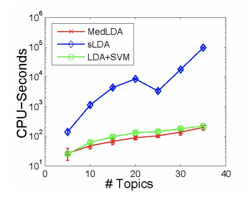
Time Efficiency

The time efficiency of MedLDA is pretty good, which is shown in Figure . It is much faster than the pure probabilistic version. Since MedLDA has some tricks that can be introduced in the optimization algorithm for the SVM + LDA.

Infinite SVM

Another example invloves exploring the large margin idea in combination with non-parametric bayesian model for classfication and feature selection. In the field of classification problems, it’s common to use mixture of classifiers. Conceptually, mixture of SVMs can be regarded as a combination of SVMs with different weights, and prefered over logistic regression since they have kernel functions. Here, we are talking about making priors over mixture of SVMs, and use infinite SVMs here.

Given the general theoretical framework of RegBayes,

\[\min _{p(\mathcal{M}), \xi} \operatorname{KL}(p(\mathcal{M}) \| \pi(\mathcal{M}))-\sum_{n=1}^N \int \log p\left(\mathbf{x}_{n} | \mathcal{M}\right) p(\mathcal{M}) d \mathcal{M}+U(\xi)\] \[\text { s.t. } : p(\mathcal{M}) \in \mathcal{P}_{\text { post }}(\xi)\]

In the case of inifite SVM:

Prior - Dirichlet process(DP)
Model - Latent class model
Likelihood - Gaussian likelihood
Posterior constraints- Max-margin constraints

Inifinite SVM is the first attempt to integrate Bayesian nonparametric, large-margin learning and kernel methods. The SVMs are treated as density functions to define likelihood of the data. The detailed process is as following.

DP mixture of large-margin classifiers. This is the process to determine which classifier to use.
Given a component classifier:
\[F(y, \mathbf{x} ; z, \eta)=\eta_{z}^{\top} \mathbf{f}(y, \mathbf{x})=\sum_{i=1}^{\infty} \delta_{z, i} \eta_{i}^{\top} \mathbf{f}(y, \mathbf{x})\]
Overall discriminant function:
\[F(y, \mathbf{x})=\mathrm{E}_{q(z, \eta)}[F(y, \mathbf{x} ; z, \eta)]==\sum_{i=1}^{\infty} q(z=i) \mathrm{E}_{q}\left[\eta_{i}\right]^{\top} \mathrm{f}(y, \mathrm{x})\]
Prediction rule:
\[y^{*}=\arg \max _{y} F(y, \mathbf{x})\]
Learning problem:
\[\min _{q(\mathbf{z}, \boldsymbol{\eta})} \mathrm{KL}\left(q(\mathbf{z}, \boldsymbol{\eta}) \| p_{0}(\mathbf{z}, \boldsymbol{\eta})\right)+C_{1} \mathcal{R}(q(\mathbf{z}, \boldsymbol{\eta}))\]

\[\mathcal{R}(q(\mathbf{z}, \boldsymbol{\eta}))=\sum_{d} \max _{y}\left(\ell_{d}^{\Delta}(y)+F\left(y, \mathbf{x}_{d}\right)-F\left(y_{d}, \mathbf{x}_{d}\right)\right)\]

With assumption and relaxation, we can make the question more easier by approximating the variational distribution:

\[q(\mathbf{z}, \boldsymbol{\eta}, \boldsymbol{\gamma}, \mathbf{v})=\prod_{d=1}^{D} q\left(z_{d}\right) \prod_{t=1}^{T} q\left(\eta_{\iota}\right) \prod_{t=1}^{T} q\left(\gamma_{\iota}\right) \prod_{t=1}^{T-1} q\left(v_{\iota}\right)\]

And the optimization can be solved with coordinate descent. For $q(\eta)$, we solve an SVM learning problem, and for $q(z)$, we get the closed update rule:

\[q\left(z_{d}=\iota\right) \propto \exp \left\{\left(\mathbb{E}\left[\log v_{t}\right]+\sum_{i=1}^{t-1} \mathbb{E}\left[\log \left(1-v_{i}\right)\right]\right)+ \rho\left(\mathbb{E}\left[\gamma_{t}\right]^{\top} \mathbf{x}_{d}-\mathbb{E}\left[A\left(\gamma_{t}\right)\right]\right)+(1-\rho) \sum_{y} \omega_{d}^{y} \mu_{t}^{\top} \mathbf{f}_{d}^{\Delta}(y)\right\}\]

Compared to infinite SVM, which is a bayesian nonparametric latent class model, infinite latent SVM is a Bayesian nonparametric latent feature/factor model, and each data point is mapped to a set of latent factors. The prior we use here is Indian Buffet process instead of a DP prior (used in infinite SVM). Nonparametric IBP prior allows the models to have an unbounded number of latent features. The regularized inference problem can be efficiently solved with an iterative procedure, which leverages existing high-performance convex optimization techniques.

The experiments showed increased performance on TRECVID2003 and Flickr image datasets.