Lecture 25: Spectral Learning for Graphical Models
Overview of the spectral learning for graphical models.
Spectral Learning for Graphical Models
Motivation
Latent variable models allows us to explicitly model the latent structure of the task, which gives us explainability in addition to learning the relationships between events. However, since latent variables are not directly observed in the data, we need to use Expectation Maximazation (EM) algorithms to learn the relationships, and that is computationally expensive.
Spectral learning is using linear algebra to learn latent variable models. Its advantages are
both theoretical…
- Provably consistent
- Deeper insight into identifiability
and practical…
- Local minima free
- 10-100x speedup over EM
- Model non-Gaussian continuous data using kernels
Spectral learning’s goal is to preserve the explanative properties and theoretical guarantees provided by latent variables, but avoid the computational cost that comes with latent variables.
We notice that in most tasks, the solution to the task itself does not require any information about latent variables - it only exists for modeling purposes.
Example: Hidden Markov Models
Let’s consider Hidden Markov Models (HMMs) as an example of a latent variable model. With latent variables, we can see that it is a computationally tractable to perform inference on HMMs since its maximum cliques are very small (size 2).
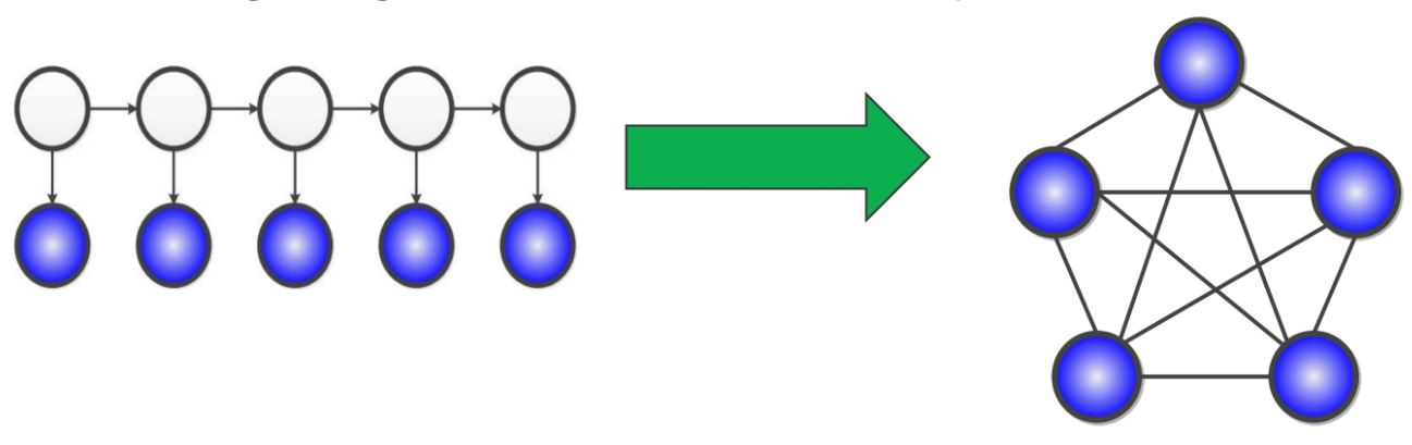
The problem arises from marginalizing out the latent (white) variables in the diagram - in the graph, we seem to arrive at a clique.
However, if looking at a simple latent variable model with one hidden, and 3 observed states depending on that hidden state, we can see that there is a relationship between the number of hidden states for $H$ and the complexity of the relationship between the observed variables once $H$ is margnialized.

If we have 1 state, then the marginal distribution is equal to the conditional distribution of the observed variables on $H$, which means they’re all independent. On the other hand if $H$ has $m^3$ states, where $m$ is the number of states for each observed variable, then the marginalization would have enough parameters to fully paramterize any relationship between the observed variables, and thus forming a clique.
Clearly, there is also an intermediate case between these two extremes - how can we exploit this relationship between observed variables?
A matrix view of probability rules
Sum Rule
- Probability form: \(\mathbb{P}[X] = \sum\limits_Y \mathbb{P}[X\mid Y]\mathbb{P}[Y]\)
- Matrix algebra form : \(\mathcal{P}[X] = \mathcal{P}[X\mid Y] \times \mathcal{P}[X]\) where $\times$ is the matrix dot product.
Chain Rule
- Probability form: \(\mathbb{P}[X, Y] = \mathbb{P}[X \mid Y]\mathbb{P}[Y] = \mathbb{P}[Y\mid X]\mathbb{P}[Y]\)
- Matrix algebra form: \(\mathcal{P}[X, Y] = \mathcal{P}[X \mid Y] \times \mathcal{P}[\mathbin Y]\) where $\mathcal{P}[Y]$ is a diagonal matrix w/ the probabilities on the diagonal.
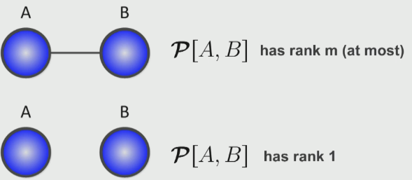
Two variable examples
If we consider a relationship between two variables $A, B$, we can observe a relationship between the ranks and the variable relationships:
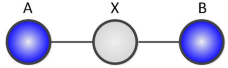
If we consider the intermediate case where we have an intermediate variable $X$ with $k$ states:
We can claim that \(rank(\mathcal{P}[A, B]) \leq k\)
Proof: We can use the matrix interpretation of the chain rule from above.
We know that
\[\mathcal{P}[A, B] = \mathcal{P}[A\mid X]\mathcal{P}[X]\mathcal{P}[B\mid X]^T\]We also note that each of these factor matrices have rank $\leq k$, which means that matrix characterizing the joint distribution must have rank $\leq k$.
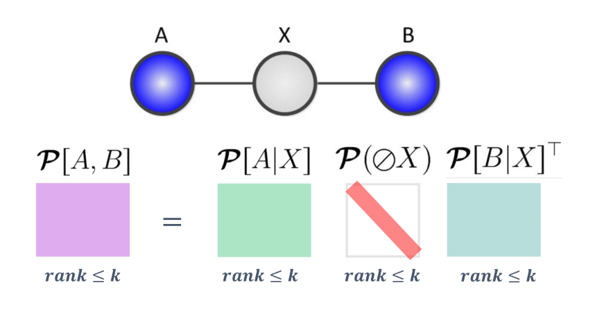
Thus, we can see that latent variable models encode low rank dependencies among variables, and we can use our linear algebra toolkit to exploit the low rank structure.
Factorization without latent variable
How to factorize with latent variables
For the above example, assume $m>k$, we can easily factorize the giant joint distribution table into several small tables by introducing latent variable $H_2$:
\[\mathcal{P}[X_{\{1,2\}}, X_{\{3,4\}}] = \mathcal{P}[X_{\{1,2\}} | H_2] \mathcal{P}[\oslash H_2]\mathcal{P}[X_{\{3,4\}}|H_2]^T\]where \(\oslash\) is means on diagonal.
The tables can be learned through EM algorithm. However, the factorization is not unique, since for any factorization \(M=LR\) we can add any invertible transformation: \(M=LSS^{-1}R\)
This insight gives us the hope that there might be some way of factorizations which do not require us to introduce any hidden variables. The magic of spectral learning is that there exist an alternative factorization that only depends on observed variables.
How to factorize without latent variables
The goal is to decompose a giant matrix $\mathcal{P}[X_{{1,2}}, X_{{3,4}}]$ into the product of several small matrices. One observation is that:
\[\mathcal{P}[X_{\{1,2\}}, X_{3}] = \mathcal{P}[X_{\{1,2\}} | H_2] \mathcal{P}[\oslash H_2]\mathcal{P}[X_{3}|H_2]^T\] \[\mathcal{P}[X_{2}, X_{\{3,4\}}] = \mathcal{P}[X_{2} | H_2] \mathcal{P}[\oslash H_2]\mathcal{P}[X_{\{3,4\}}|H_2]^T\]It can be seen that for the terms on the right hand sides of the above equations,
\[\mathcal{P}[X_{\{1,2\}} | H_2] \mathcal{P}[\oslash H_2]\mathcal{P}[X_{\{3,4\}}|H_2]^T = \mathcal{P}[X_{\{1,2\}}, X_{\{3,4\}}]\] \[\mathcal{P}[X_{2} | H_2] \mathcal{P}[\oslash H_2]\mathcal{P}[X_{3}|H_2]^T=\mathcal{P}[X_{2}, X_{3}]\]which leads to: \(\mathcal{P}[X_{\{1,2\}}, X_{\{3,4\}}] = \mathcal{P}[X_{\{1,2\}}, X_{3}]\mathcal{P}[X_{2}, X_{3}]^{-1}\mathcal{P}[X_{2}, X_{\{3,4\}}]\)
which gives a factorization that only contains observed variables, indicating there is no need to learn latent variables using EM, hence it is more efficient an no local optimal problem. The caveat is that \(\mathcal{P}[X_{2}, X_{3}]\) have to be invertible. We call this factorization observable factorization.
There are also other ways of observable factorization, e.g. \(\mathcal{P}[X_{\{1,2\}}, X_{\{3,4\}}] = \mathcal{P}[X_{\{1,2\}}, X_{4}]\mathcal{P}[X_{1}, X_{4}]^{-1}\mathcal{P}[X_{1}, X_{\{3,4\}}]\)
By “combining” different observable factorizations, we might do better empirically.
Relationship between observable factorization and factorization with latent variable
Let \(M := \mathcal{P}[X_{\{1,2\}}, X_{\{3,4\}}]\) \(L := \mathcal{P}[X_{\{1,2\}} | H_2] \mathcal{P}[\oslash H_2]\) \(R := \mathcal{P}[X_{\{3,4\}}|H_2]^T\) The original factorization with latent variables can be represented as \(M = \mathcal{P}[X_{\{1,2\}} | H_2] \mathcal{P}[\oslash H_2]\mathcal{P}[X_{\{3,4\}}|H_2]^T=LR\)
Let \(S:=\mathcal{P}[X_3|H_2]\) Then
\(LS = \mathcal{P}[X_{\{1,2\}}, X_{3}]\) \(S^{-1}R = \mathcal{P}[X_{2}, X_{3}]^{-1}\mathcal{P}[X_{2}, X_{\{3,4\}}]\) Therefore, the observable factorization can be represented as: \(M=\mathcal{P}[X_{\{1,2\}}, X_{\{3,4\}}] = \mathcal{P}[X_{\{1,2\}}, X_{3}]\mathcal{P}[X_{2}, X_{3}]^{-1}\mathcal{P}[X_{2}, X_{\{3,4\}}]=LSS^{-1}R\)
Training / Testing with Spectral learning
training
For observable factorization: \(\mathcal{P}[X_{\{1,2\}}, X_{\{3,4\}}] = \mathcal{P}[X_{\{1,2\}}, X_{3}]\mathcal{P}[X_{2}, X_{3}]^{-1}\mathcal{P}[X_{2}, X_{\{3,4\}}]\)
we can simply obtain MLE of the matrices on the right hand side by counting from samples.
testing
To compute the probability of a observed data $(x_1,x_2,x_3,x_4)$, we can simply plug in the data into the MLE of the matrices:
\[\hat{\mathcal{P}}_{spec}[X_{\{1,2\}}, X_{\{3,4\}}] = \mathcal{P}_{MLE}[X_{\{1,2\}}, X_{3}]\mathcal{P}_{MLE}[X_{2}, X_{3}]^{-1}\mathcal{P}_{MLE}[X_{2}, X_{\{3,4\}}]\]Consistency
Consistency means with the increase of the sample size, the joint probability table should converge in probability to the real joint distribution.
trivial estimator
A trivial estimator is to simply estimate the big probability table from data by naive counting: \(\mathcal{P}_{MLE}[X_1,X_2;X_3,X_4] \rightarrow \mathcal{P}[X_1,X_2;X_3,X_4]\) which is consistent but statistically inefficient.
factorization with latent variables
The estimator based on factorization with latent variables are given by EM, which will get stuck in local optima and is not guaranteed to obtain the MLE of the factorized model.
\[\mathcal{P}_{MLE}[X_{\{1,2\}} | H_2] \mathcal{P}_{MLE}[\oslash H_2]\mathcal{P}_{MLE}[X_{\{3,4\}}|H_2]^T \rightarrow \mathcal{P}[X_1,X_2;X_3,X_4]\]Spectral learning
Spectral learning estimator is consistent and computationally tractable, at some loss of statistical efficiency due to the dependence on the inverse.
\[\mathcal{P}\mathcal{P}_{MLE}[X_{\{1,2\}}, X_{3}]\mathcal{P}_{MLE}[X_{2}, X_{3}]^{-1}\mathcal{P}_{MLE}[X_{2}, X_{\{3,4\}}] \rightarrow \mathcal{P}[X_1,X_2;X_3,X_4]\]Conditional tree latent models
Factorization can be applied to tree models as well, by creating triplets of parameters that are represented by tensors. Further reading on these case studies are (Song et al.) and (Parikh et al.).
When Does the Inverse Exist
\(\mathcal{P}[X_2, X_3] = \mathcal{P}[X_2 | H_2] \mathcal{P}[\oslash H_2]\mathcal{P}[X_3|H_2]^T\)
In order for the probability matrix on the left hand side invertible, all the matrices in the right hand side must have full rank. (This is a in general a requirement for spectral learning, although it can be somewhat relaxed.)
Given the case that the dimension of the hidden state is $k$ and the dimension of the output variable is $m$, we discuss the following senarios.
- When $m > k$ The inverse cannot exist, but this situation is easily fixable by projecting the matrix into a lower dimensional space.
where $U, V$ are the top left/right k singular vectors of $\mathcal{P}[X_2, X_3]$.
- When $k > m$ The inverse does exist. But it no longer satisfies the following property, which we used to derive the factorization.
This is much more difficult to fix, and intuitively corresponds to how the problem becomes intractable if $k \gg m$.
* Intuitively, larger $k$ and smaller $m$ means long range dependencies.
* Consider the following generative process:
    (1) With probability 0.5, let $S=X$, and with probability 0.5, let $S=Y$.
    (2) Print A $n$ times.
    (3) Print S.
    (4) Go back to step (2)
* With $n=1$ we either generate AXAXAX.... or AYAYAY....
  With $n=2$ we either generate AAXAAXAA.. or AAYAAYAA..
* HMM needs $2n$ states to to remember count as well as whether we picked $S=X$ or $S=Y$. However, number of observed states $m$ does not change, so our previous spectral algorithm will break for $n>2$.
* How can we deal with this in spectral framework?
Making Spectral Leanring Work in Practice
-
We are only using marginals of pairs/triples of variables to construct the full marginal among the observed variables, which only works for the case of $k<m$. However, in real problems we need to capture longer range dependencies.
-
Recall our factorization
In order to use long-range features, we can construct feature vector of the left side $\phi_L$ and the feature vector $\phi_R$ of the right side.
- Spectral Learning with Features
We can use more complex features to replace $\delta_2 \otimes \delta_3$. And $\mathcal{P}[X_{{1, 2}}, X_{{3, 4}}]$ can be represented as follows: \(\mathcal{P}[X_{\{1, 2\}}, X_{\{3, 4\}}] = \mathbb{E}[\delta_{1 \otimes 2}, \delta_{3 \otimes 4}] = \mathbb{E}[\delta_{1 \otimes 2}; \phi_R] V (U^T \mathbb{E}[\phi_L \otimes \phi_R] V)^{-1} U^T \mathcal{P}[\phi_L, X_{\{3, 4\}}]\)
Experimental Results
Experimentally, it’s been shown by many authors that spectral methods achieve comparable results to EM but are 10-50X faster(Parikh et al. 2011, Parikh et al. 2012, Balle et al. 2012, Cohen et al. 2012, Cohen et al. 2013). We show some synthetic and real data results demonstraing the comparison between EM and spectral methods.
- Synthetic data (Parikh et al. 2012)
- A novel representation of latent variable models (junction tree specifically)
- Train: Learn parameters of a given model given samples of observed variables.
- Test: Evaluate likelihood of random samples drawn from model and compare to the true likelihood
- Synthetic 3rd order HMM example (Spectral/EM/Online EM). Results of other sturctures are similar. We can see that the running time of spetral methods is less than that of Online EM and EM algorithms while the error rate keeps low.

- Supervised Parsing (Cohen et al. 2012/2013)
- Learn a latent variable Prbabilistic Context Free Grammar (latent PCFG) which is a PCFG augmented with additional latent states.
- Train: Learn parameters given parse trees on training examples
- Test: Estimate most likely parse structure on test sentences
- Empirical results for latent PCFGs
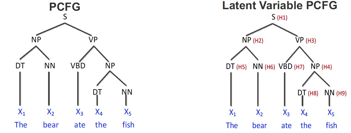
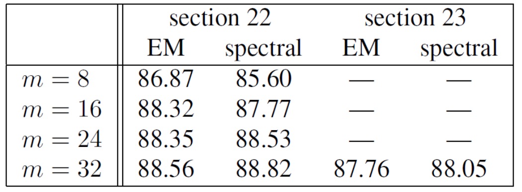
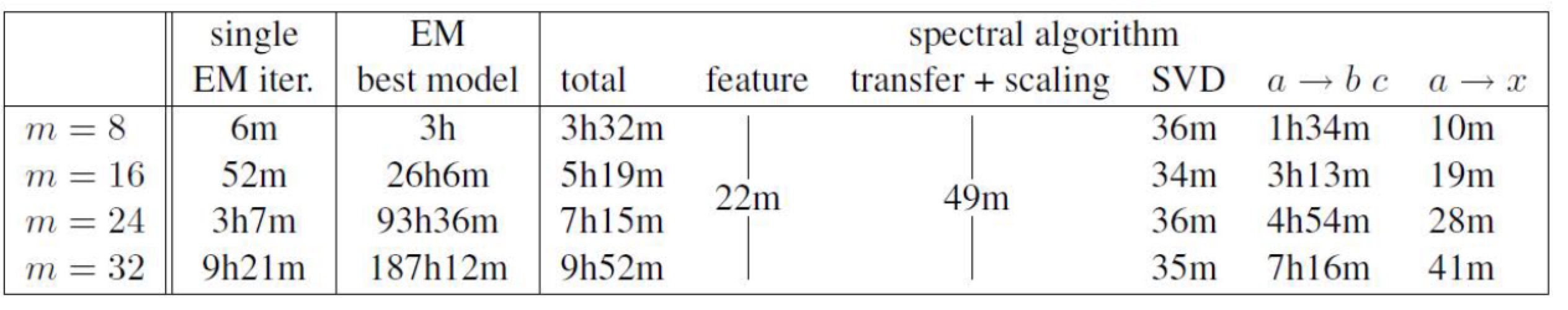
It shows that the results of spectral learning are at least comparable to EM algorithms. But the speed is much faster.
Connection to Hilbert Space Embeddings
- Dealing with Nonparametric Continuous Variables
- It is difficult to run EM if the conditional/marginal distribution are continuous and do not easily fit into a parametric family.
- However, we will see that Hilbert Space Embeddings can easily be combined with spectral methods for learning nonparametric latent models.
- Recall that we could substitute features for variables
We can replace $\mathcal{P}[X_2, X_3]$ with
\[\mathcal{C}[X_2, X_3] = \mathbb{E}[\phi_{X_2} \otimes \phi_{X_3}]\]- Therefore, with discrete case, we have
and with continuous case, we have
\[\mathcal{C}[X_{\{1, 2\}}, X_{\{3, 4\}}] = \mathcal{C}[X_{\{1, 2\}}, X_3]\mathbf{V}(\mathbf{U}^T \mathcal{C}[X_2, X_3]V)^{-1}U^T \mathcal{C}[X_2, X_{\{3, 4\}}]\]Summary - EM & Spectral
| EM | Spectral |
|---|---|
| Aims to find MLE, so more “statistically” efficient | Does not aim to find MLE, so less “statistically” efficient |
| Can get stuck in local optima | Local optima free |
| Lack of theoretical guarantees | Provably consistent |
| Slow | Very fast |
| Easy to derive for new models | Challenging to derive for new models (Unknown whether it can generalize to arbitrary loopy models) |
| No issues with negative numbers | Problems with negative numbers. Requires explicit normalization to compute likelihood |
| Allows for easy modelling with conditional distributions | Allows for easy modelling with marginal distributions |
| Difficult to incorporate long-range features (since it increases treewidth) | Easy to incorporate long-range features |
| Generalizes poorly to non-Gaussian continuous variables | Easy to generalize to non-gaussian continuous variables via Hilbert Space Embeddings |