Lecture 28: A Civil Engineering Perspective on AI

Industrialization of AI

Barriers to AI Solutions Today

According to a McKinsey CEO survey in 2018, only 39% of the companies made significant progress in implementing AI applications. Up to 7% of the companies made no progress.

A Result of McKinsey CEO Survey

In addition, according to the survey, top barriers to AI applications are lack of talent and knowledge as well as AI technology and maturity.

To develop their AI applications, the companies need to either build their own AI systems or deploy their applications on a third-party platform. However, issues exist on both paths:

• Building is infeasible
  • Scarce resources in data scientists, ML engineers and system engineers
  • Little or no enterprise support from open source software
  • Major infrastructure requirements not satisfied
  • Long development timelines
  • High delivery risks
• Lack of viable third-party platform
  • Limited to cloud deployment
  • Limited customization
  • Limited service
  • Limited scalability
  • Limited capabilities

Inter-operability between diverse systems

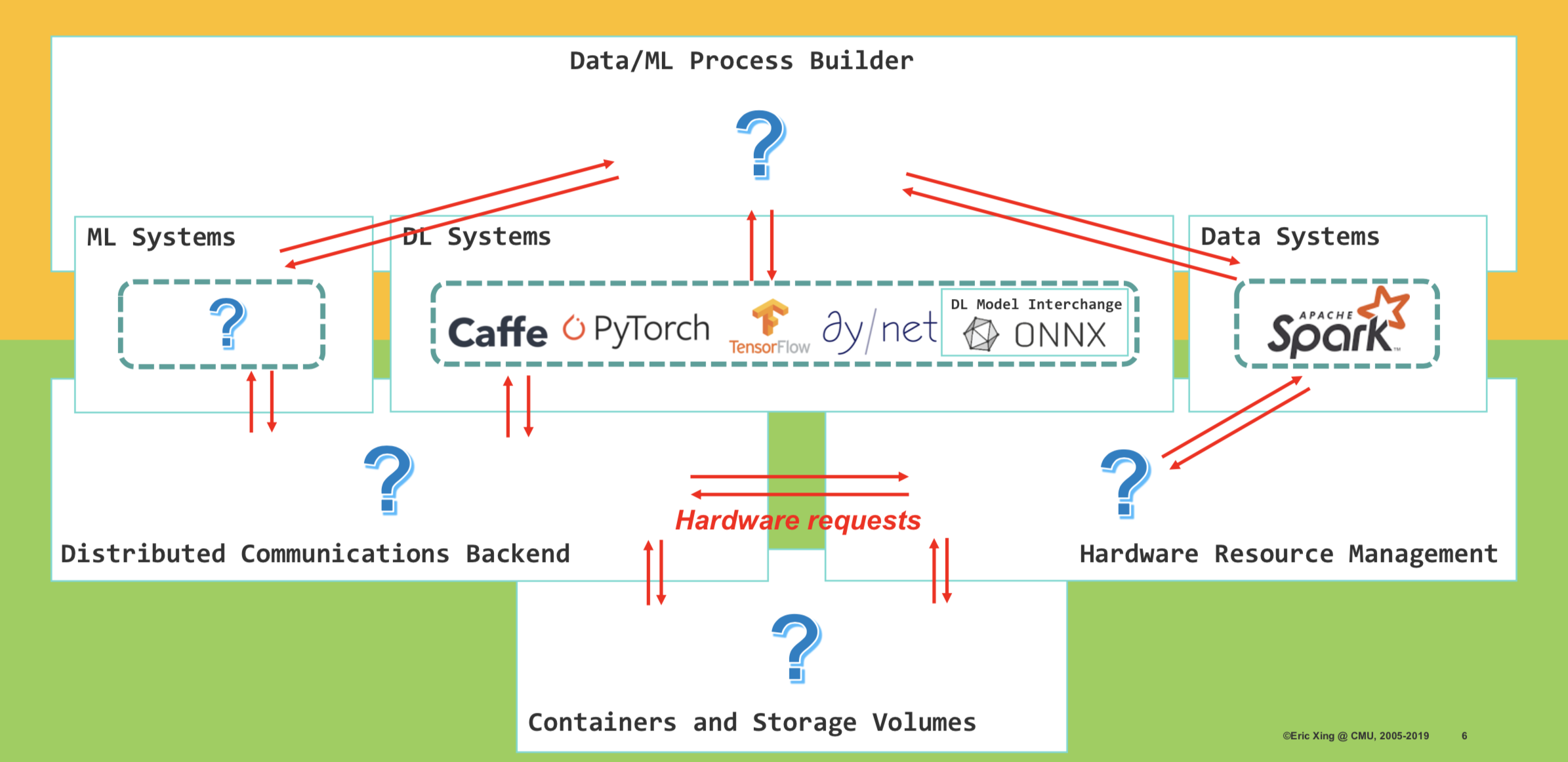
Inter-operability between diverse systems is another main concern when developing AI applications. As shown in the figure above, there are many communications between systems:

• Communications between Data/ML Process Builder and ML Systems/DL Systems/Data Systems
• Communications between Distributed Communications Backend and ML Systems/DL Systems
• Communications between Hardware Resource Management Module and Data Systems
• Communications between Containers & Storage Volumes and Hardware Resource Management Module
• Communications between Containers & Storage Volumes and Distributed Communications Backend

Transforming AI into Civil Engineering

Duty of a AI System Builder:

• Build
  • Build a full, engineering-wise sound solution, not a toy or a demo
  • Create Many copies
  • Build at low expense
  • Satisfy any client-specified conditions
• Understand
  • Understand how a solution is built
  • Understand the feasibility of proposed solutions
  • Explain why the solution works and why not if undesirable outcome
• Sustain
  • Operationalize the solution (deploy, train, etc.)
  • Guarantee reproducible results
  • Teach others to build the solution and reproduce the result

New generation of AI programs should be:

• Reusable: pluggable modules allowing enterprises to architect and customize AI rapidly
• Standard: instruction sets and pre-built functions ensuring outcomes are reproducible and sound
• Comprehensive: inventory of ML/System nuts and bolts meeting the needs for any data type, wide range of tasks, commodity hardware, and mission sizes.

Designing ML systems with first principles

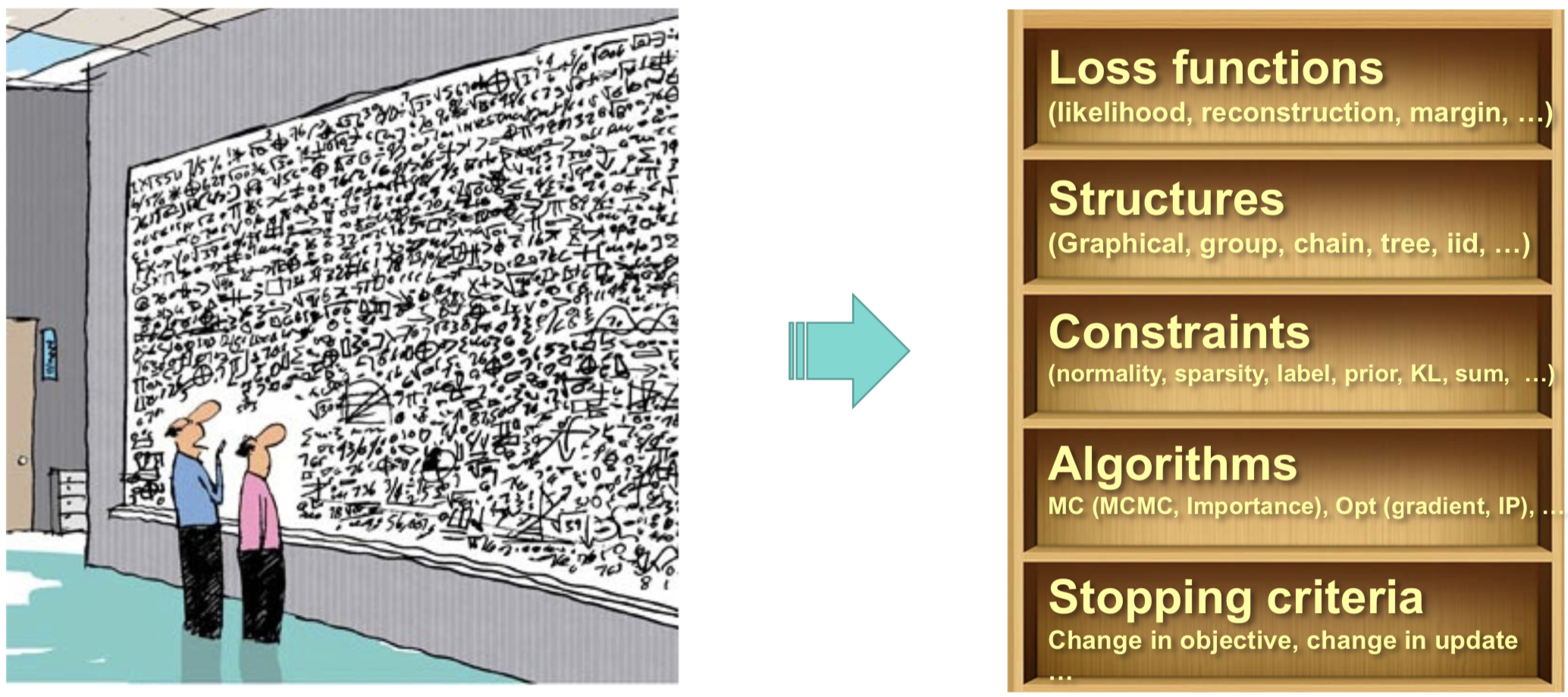
First principles:
To enable such a transformation of AI into civil engineering, principled ML process is required. First principles are sound, explainable and verifiable. Consider the figure above. According to first principles, instead of mixing everything together in a ML system, we should first explicitly define components of a ML process and then incorporate different techniques to implement the components. E.g., we choose a margin loss as our loss function. we choose neural network as our model structure. We use sparsity constraints in the objective function. We use gradient descent as our algorithm to solve the problem. We observe the change of value of objective function to decide when to stop.

Basic ML principles: Consistency, Bias v/s variance, Sample complexity, Learning rate, Convergence, Error bound, Confidence, Stability, etc..

Relations among ML principles in PAC Learning Theory

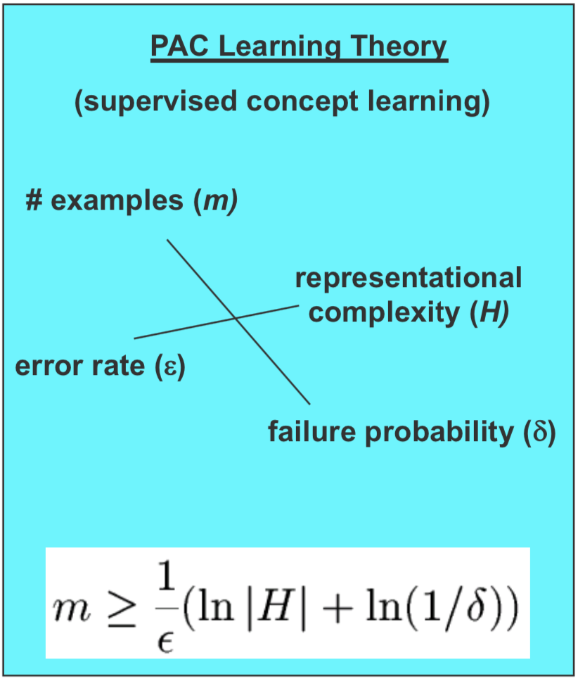
An example of managing different ML principles exists in Probably Approximately Correct (PAC) Learning Theory. Sample size $m$, representational complexity $H$, error rate $\epsilon$ and failure probability $\delta$ satisfy the following inequality:

\[m \geq \frac{1}{\epsilon}(ln|H|+ln(\frac{1}{\delta}))\]

Loss Augmentation:
In Bayesian Learning, distribution parameters $\theta$ is treated as a random variable. According to Bayes’ Rule, the posteriori distribution of $\theta$ after data is seen is:

\[p(\theta \mid D) = \frac{p(D \mid \theta)p(\theta)}{p(D)} = \frac{p(D \mid \theta)p(\theta)}{\int p(D \mid \theta)p(\theta)d\theta}\]

In Frequentist Regularization, parameter $\theta$ is treated as an unknown constant. The regularized estimate of $\theta$ after data is seen is:

\[\mathop{\arg\max}\limits_{\theta} = \mathcal{L}(\{x_i, y_i\}_{i=1}^{N};\theta) + \Omega(\theta)\]

The prior of $\theta$ $p(\theta)$ in Bayesian Learning, or the regularizer $\Omega(\theta)$ in Frequentist Regularization, encodes our prior knowledge about the domain.

Inference Methods:
In Variational Inference, we want to infer the distribution of latent variable $Z$ given the observable variable $X$ by maximizing the expectation of the log probability of $X$ under the posterior of $Z$.

\begin{aligned} \mathbb{E}_{q_\phi(z \mid x)} log p(x) &= \int q_\phi(z \mid x)logp(x)dz \\ &= \int q_\phi(z \mid x)log\frac{p_\theta(x, z)}{p_\theta(z \mid x)}dz \\ &= \int q_\phi(z \mid x)log\frac{p_\theta(x, z)}{q_\phi(z \mid x)}\frac{q_\phi(z \mid x)}{p_\theta(z \mid x)}dz \\ &= \int q_\phi(z \mid x)log\frac{p_\theta(x, z)}{q_\phi(z \mid x)}dz + \int q_\phi(z \mid x)log\frac{q_\phi(z \mid x)}{p_\theta(z \mid x)}dz \\ &= KL(q_\phi(z \mid x) || p_\theta(z \mid x)) + \mathbb{E}_{q_\phi(z \mid x)} log\frac{p_\theta(x, z)}{q_\phi(z \mid x)} \end{aligned}

As shown above, since $KL(q_\phi(z \mid x) || p_\theta(z \mid x)) \geq 0$, we have the lower bound of the true objective function
is:

\[\mathcal{L}(\theta, \phi;x) = \mathbb{E}_{q_\phi(z \mid x)} log\frac{p_\theta(x, z)}{q_\phi(z \mid x)}\]

We maximize this variational lower bound of the true objective function instead, or equivalently, minimize the free energy

\[F(\theta, \phi;x) = -\mathbb{E}_{q_\phi(z \mid x)} log p(x) + KL(q_\phi(z \mid x) || p_\theta(z \mid x))\]

.We further transform the variational lower bound as the following:

\begin{aligned} \mathcal{L}(\theta, \phi;x) &= \int q_\phi(z \mid x)log\frac{p_\theta(x, z)}{q_\phi(z \mid x)}dz \\ &= \int q_\phi(z \mid x)log\frac{p_\theta(x \mid z)p(z)}{q_\phi(z \mid x)}dz \\ &= \int q_\phi(z \mid x)log p_\theta(x \mid z)dz + \int q_\phi(z \mid x)log\frac{p(z)}{q_\phi(z \mid x)}dz \\ &= \mathbb{E}_{q_\phi(z \mid x)} log p_\theta(x \mid z) - \int q_\phi(z \mid x)log\frac{q_\phi(z \mid x)}{p(z)}dz \\ &= \mathbb{E}_{q_\phi(z \mid x)} log p_\theta(x \mid z) - KL(q_\phi(z \mid x) || p(z)) \end{aligned}

E-step: We maximize $\mathcal{L}(\theta, \phi;x)$ w.r.t. $\phi$ with $\theta$ fixed.
M-step: We maximize $\mathcal{L}(\theta, \phi;x)$ w.r.t. $\theta$ with $\phi$ fixed.

Demistifying and Unifying different models:
As an example, we want to unifying the zoo of Deep Generative Models (DGMs): GANs, VAEs, WS, VI, etc..

Commonness: All with implicit distributions and black-box Neural Network models in terms of the formulation.
Difference: Different space complexity and loss functions, e.g., GAN uses an adversarial loss while VAE uses a maximum likelihood loss.

Designing proper model/algorithms with Guarantees:
Assume we solve a regression problem as the following:

\[\mathop{\arg\max}\limits_{\theta} = \mathcal{L}(\{x_i, y_i\}_{i=1}^{N};\theta) + \Omega(\theta)\]

To provide an algorithm with guarantees, we use an iterative-convergent gradient algorithm as the following:

\[\theta^{(t)} = \theta^{(t-1)} + \epsilon\nabla\mathcal{L}(\theta^{(t-1)}, D^{(t)})\]

Good Generalizability of models:

Models with different generalizability

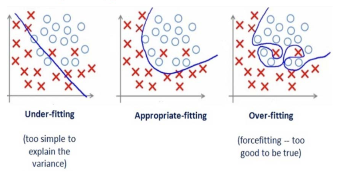
We should avoid our models from underfitting and overfitting.

Case Analysis: Medical Imaging Report Generation
In traditional way of generating imaging report, the radiology observations and findings regarding each area of the body are first examined in the imaging study, then the findings, the patient clinical history and the indication for the imaging study are combined to provide a diagnosis.

However, there are difficulties in Automatic Imaging Report Generation:

• Abnormal regions in medical images are difficult to identify.
• The reports are typically long, containing multiple sentences.
• Each sentence discusses a specific topic so localization of the image regions and tags that are relevant to this topic is required.

Models with different generalizability

Several models and techniques are used here:

• Semi-supervised learning for lesion tag prediction.
• Hierarchical LSTM for long-paragraph generation.
• Visual-semantic co-attention to localize the relevant image regions and tags for each sentence to be generated.

Building v/s Crafting:
To realize AI version of civil engineering, understanding the term of “building” is extremely important. Building entails the design of the system structure, the plan of building the system, the budget for the system, the requirement for materials (data, knowledge, infrastructure, etc.), the methods used in the system, the implementation details, the integration of different modules, the refinement/tuning of the system to get optimal performance, the deployment of the system on other platforms, the test of the system under normal and stress case, the maintenance and upgrade of the system and the security of the system.

Case Analysis: Solving a ML Program
Assume we are solving a Machine Learning Program as the following. Our model is represented in the objective, our data is $y$ and our parameter is $\theta$.

\[\mathop{\arg\max}\limits_{\theta} = \mathcal{L}(\{x_i, y_i\}_{i=1}^{N};\theta) + \Omega(\theta)\]

We use an iterative convergent algorithm to solve it, usually Gradient Descent as the following.

\[\theta^{(t)} = \theta^{(t-1)} + \eta\nabla\mathcal{L}(\theta^{(t-1)})\]

However, if the regularizer is not differentiable (e.g., L-1 norm), we cannot use gradient descent here. Here is how Proximal Gradient Descent comes into place.

\begin{aligned} v^{(t)} &\leftarrow \theta^{(t-1)} - \eta\nabla_{\theta^{(t-1)}}\mathcal{L}(\theta^{(t-1)}) \\ \theta^{(t)} &\leftarrow \mathop{\arg\min}\limits_{z}\frac{1}{2\eta}||v^{(t)} - z||^{2} + \Omega(z) \end{aligned}

Here $\mathop{\arg\min}\limits_{z}\frac{1}{2\eta}||\theta^{(t)} - z||^{2} + \Omega(z)$ is the proximal map for $\theta$. For every iteration, we first compute the gradient of
$\theta$, and then projected $\theta$ onto the proximal map. The time complexity of Proximal Gradient Descent is $O(1/\eta t)$.

To accelerate Proximal Gradient Descent, we have an accelerated version, which is also called Fast Iterative Shrinkage-Thresholding Algorithm (FISTA).

\begin{aligned} v^{(t)} &\leftarrow \theta^{(t-1)} - \eta\nabla_{\theta^{(t-1)}}\mathcal{L}(\theta^{(t-1)}) \\ u^{(t)} &\leftarrow \mathop{\arg\min}\limits_{z}\frac{1}{2\eta}||v^{(t)} - z||^{2} + \Omega(z) \\ \theta^{(t)} &\leftarrow u^{(t)} + \frac{t-1}{t+2}(u^{(t)} - u^{(t-1)}) \end{aligned}

As shown above, for every iteration, the first two steps of the algorithm is the same with Proximal Gradient Descent. At the third step, the momentum is considered to update $\theta$. With acceleration, the time complexity is boosted to $O(1/\eta t^2)$.

To use Moreau envelope as smooth approximation of the objective of Proximal Gradient Descent has a rich and long history in convex analysis. Inspired from proximal point algorithm, which is exactly the second step for every iteration of Proximal Gradient Descent, an approximation of the objective is given as the following:

\[\min\limits_{\theta} \mathcal{L}(\theta) + \Omega(\theta) \approx \min\limits_{\theta} M_{\mathcal{L}}^{\eta}(\theta) + \Omega(\theta)\]

The Smooth Proximal Gradient Descent first computes the proximal map of the last $\theta$ on the differentiable part of the objective, and then computes the proximal map of the result of the first step on the non-differentiable part. Finally, it applies the momentum similar to Accelerated Proximal Gradient Descent.

\begin{aligned} v^{(t)} &\leftarrow \mathop{\arg\min}\limits_{z}\frac{1}{2\eta}||\theta^{(t-1)} - z||^{2} + \mathcal{L}(z) \\ u^{(t)} &\leftarrow \mathop{\arg\min}\limits_{z}\frac{1}{2\eta}||v^{(t)} - z||^{2} + \Omega(z) \\ \theta^{(t)} &\leftarrow u^{(t)} + \frac{t-1}{t+2}(u^{(t)} - u^{(t-1)}) \end{aligned}

Data-Parallel for large-scale problems:

Models with different generalizability

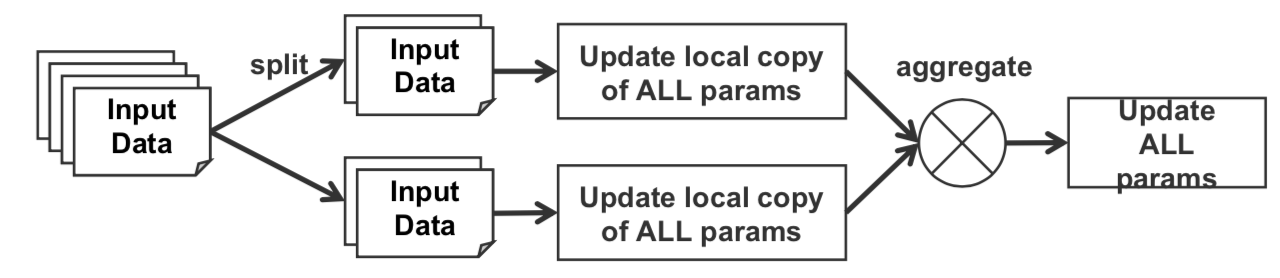
If data is too large to fit in a single worker, divide it among P workers. For every iteration, each worker receives a stale sub-updates and all the sub-updates are aggregated to get the total update.

Modularization and Standardization

Our goal is to systematically order the nuts and bolts so that we can easily pick the components we need. There are three stages of nuts and bolts:

\begin{itemize} \item Data wrangling: projections, transformations and embeddings of data \item Machine learning: loss functions, regularizers/priors, training algorithms \item System harmonization: distributed ML, parameter servers \end{itemize}

Each stage can be further broken down into steps. Data wrangling steps are ingestion, cleaning and improvement, feature engineering, embedding, and integration. Machine learning steps are build, augment and tune, train, score, and experiment. The steps for system harmonization are deploy, storage, compatibility, user accounts and security, and project management.

Interoperability

There should be standards for interfaces between nuts and bolts so that any algorithm can be used after any data wrangling method.

Process

There should be a workbench where people can easily create, experiment, explain and manage their tasks. A graphical interface may be useful for this process.

Soundness

If you have correctly modularized and implemented components, then you guarantee soundness of the system. You can use the theory and guarantees for each component to build the guarantees for the whole system.

Real-World Example: Texar

Texar is a toolkit for text generation built on these principles.

Language model example

A language model computes the probability of a sentence $y = (y_1, y_2,….y_T)$ as $p_\theta(y) = \prod_{t=1}^T p_{\theta}(y_t \mid y_{t-1})$ according to the Markov assumption. In the simplest case, we can use an HMM to model this. We can allow more dependences by letting each hidden state be an LSTM. We can incorporate additional context by using a conditional language model that computes the conditional probability of a sentence $p_\theta(y \mid x) = \prod_{t=1}^T p_{\theta}(y_t \mid y_{t-1}, x)$. The language model can be viewed as a decoder and the context can be modeled as an encoder. With this formulation, we can plug in many different options into the encoder.

Reinforcement learning

We can use reinforcement learning to create a closed loop between data sampling and evaluation that allows us to continuously train. For instance, if our test metric is BLEU, and we have a decoder that generates samples $\hat{y}$ which are used to evaluate the reward, then we can use a reinforcement learning process that automatically updates the decoder based on the BLEU metric after we sample a $\hat{y}$.

The key idea is that the model should be modular and composable; instead of building from scratch, we should be assembling composable parts.

Distributed Machine Learning

You might have noticed that this year was the first SysML conference (last year’s SysML was just a workshop). The goal of this new conference is to promote the co-design of machine learning systems and machine learning algorithms. One interesting area at the intersection of ML and systems is distributed machine learning. When implementing ML algorithms in a distributed system, there are a lot of interesting questions that arise such as which quantities to transfer between the machines, how often to transfer those quantities, etc.

In this lecture, we’ll discuss two interesting architectures for distributed machine learning: the parameter server architecture and the sufficient vector architecture.

Parameter servers and bounded asynchrony

Suppose that you’re trying to train an ML model on a huge dataset, and you have many machines at your disposal. One natural idea is to shard the data across many worker machines, but store the whole model on a single master machine called the parameter server (in practice, the PS could also be group of machines if the model is too big to fit on a single machine).

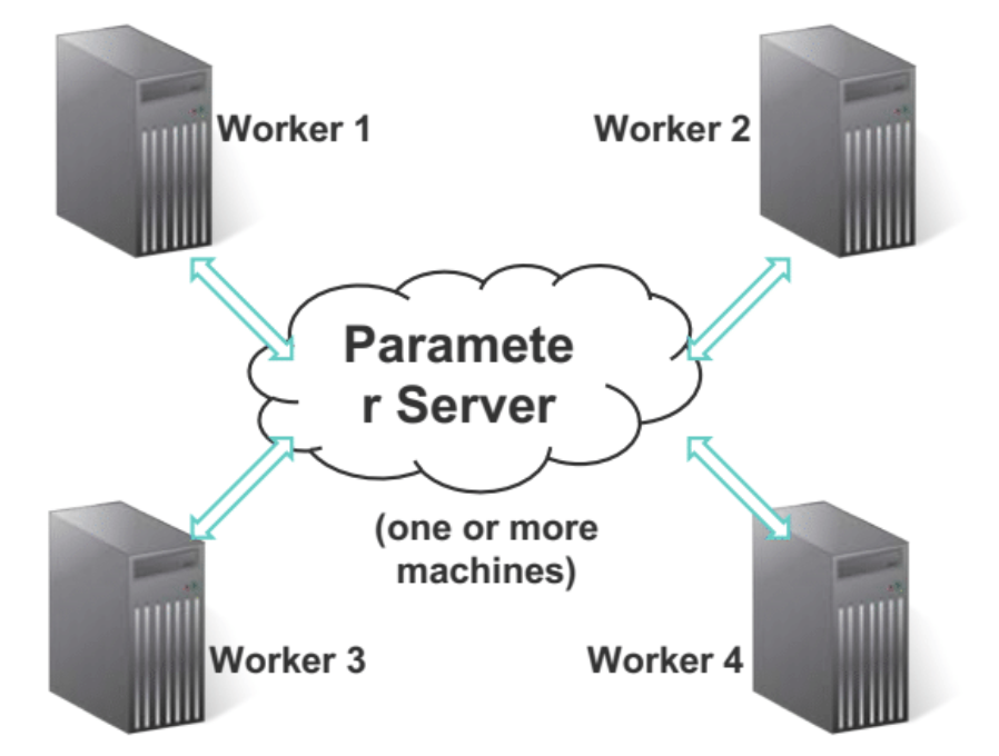
(Interestingly, a very simple instance of the parameter server architecture occurs where you have a single machine with multiple worker threads accessing a model stored in shared memory.)

In the most naive PS architecture, each worker retrieves the latest copy of the model from the master / parameter server, then computes model updates using its own subset of the dataset, and then sends its model update back to the master/parameter server, which aggregates all worker’s updates.

One problem with this naive architecture is that there might be stragglers — some workers might take longer to compute their updates, and it’s inefficient force the remaining workers to wait for the straggler to get its updates in. The solution to this straggler problem is to permit some degree of asynchrony — model parameters are dispatched asynronously to the workers, before all workers’ model updates from the previous iterataion are in. The trick to making this work is to enforce that the amount of asynchrony is bounded. With bounded asynchrony, you can prove convergence theorems. For example, Theorem 5 in proves that the difference between the current iterate’s objective value and the optimal objective value decreases exponentially. Notice that this bound depends explicitly on the expectation and variance of the delay between all workers in the cluster. These two numbers can be controlled by the operator of the system.

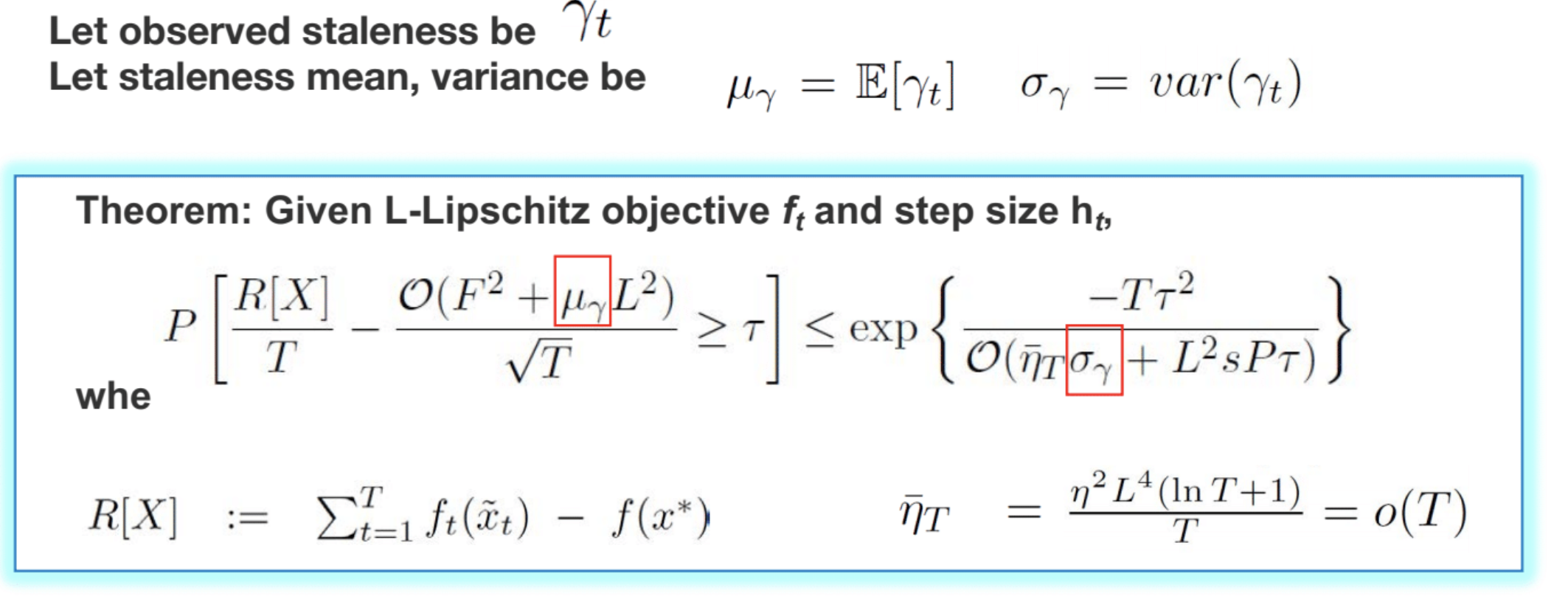
This theorem was the first of its kind when it was published in 2013. It was unique because it modeled parameters of the system. Usually, ML theorems just make assumptions about the smoothness of a function or the properties of the data. But that type of theorem is not very useful in practice, because real computer systems can behave in very strange ways. This theorem is interesting because it brings parameters of the real computer system into the analysis.

Sufficient factor broadcasting

The trouble with the parameter server architecture is that it requires the whole model to be transmitted between each worker, and the parameter server, in every iteration. This is infeasible for huge models like DNNs which may be gigabytes in size. Fortunately, it turns out that for a certain class of models called matrix parameterized models, you can get away with just passing around a low-rank version of the model updates between the workers. This approach is called sufficient factor broadcasting.

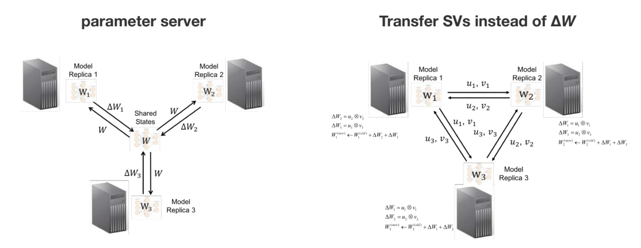
In sufficient factor broadcasting, you do not have a parameter server which is the ground source of truth for the model weights. Instead, each worker maintains its own copy of the model weights. In every iteration, each worker sends the model updates, computed over its subset of the dataset, as a message to every other worker. Now, it may seem at first as if this is completely impractical – if you do this in the naive way, the model update \(\Delta W\) is just as large as the model itself!

However, it turns out that for so-called matrix parameterized models, each model update is low-rank, so rather than passing around the full update, each worker can just send the other workers the low rank factors.

Matrix-parameterized models take the following form:

\[\min_W \frac{1}{N} \sum_{i=1}^N f_i (W a_i) + h(W)\]

where \(h\) is a regularizer and \(f_i\) is the loss for the \(i\)-th data point (which may, for example, implicitly depend on that data point’s label).

Examples of MPMs include distance metric learning, multi class logistic regression, topic models, sparse coding, neural networks, etc. In multiclass logistic regression, the rows of the parameter matrix are the coefficient vectors for the different classes; in sparse coding, the rows of the parameter matrix are the basis vectors used to reconstruct the observed data.

The trick behind the sufficient factor broadcasting framework is that the SGD update in a matrix-parameterized model is low-rank:

\[\Delta W = u v^T \quad u = \frac{\partial f(W a_i)}{\partial (W a_i)} \quad v = a_i\]

Therefore, rather than passing around \(\Delta W\), you can just pass around \(u\) and \(v\).

Interestingly, it’s not only the SGD update that’s low-rank: the SDCA update is also low-rank.

This paper provides a detailed analysis of the correctness of this approach. Interestingly, it turns out that each machine doesn’t need to send its updates to every other worker, only to its nearest neighbors. You can prove that the result you get from this protocol is equivalent, under certain conditions, to the result you’d get if you broadcasted the updates to every other worker.

Parameter Server / Sufficient Factor Hybrid

The parameter server idea and the sufficient factor idea can be combined. For example, if you’re training a neural network, note that the parameters for the early, convolutional layers take up way less space than the parameters for the later, fully-connected layers. Therefore, you can transmit the convolutional parameters using a parameter server master/slave setup (each worker sends its weight update to the master server, which sends to all the workers), while you can transmit the fully-connected parameters using a peer-to-peer sufficient factor setup.

Programming Interfaces and Software Frameworks

Another exciting research direction at the intersection of systems and machine learning are programaming interfaces and software frameworks for deep learning, such as Cavs, a DL framework recently developed by Petuum.

Modern DL frameworks are either static graphs, like TensorFlow, or dynamic graphs, like PyTorch. The advantage of the static graph approach is that you can optimize the computational graph. However, the disadvantage is that it’s hard for frameworks based on static graphs to handle inputs of variable length, such as sentences with variable number of words or images with a variable size. You have to resort to hacks like zero-padding all sentences to be the length of the largest possible sentence, or creating a number of different static graphs, one for each possible sentence length.

Cavs takes a different approach, inspired by graph processing software frameworks. Graph-processing software often follows a vertex-centered approach called vertex programming. In vertex programming, the programmer defines each vertex’s role, in terms of its inputs from neighboring vertices and its outputs to neighboring vertices.

In Cavs, the programmer writes a vertex program, which is optimized. However, at runtime, the graph that is fed to the vertex program can be of any size. Cavs therefore gives the best of both worlds — the optimizations of a static graph, but without the hasslse.

As you can see from the comparison below, Cavs (green bars) is much faster than TensorFlow (brown bars):

Explainable AI

Explainability is an important area of research/engineering these days. It’s important to keep in mind that explainability is not just about showing the weights of the model. There are several different types of explainability that are equally important:

• Data explainability: how the data is processed
• Model explainability: what you’ve learned, e.g. feature weights
• Inference explainability: how each result is inferred
• Process explainability: factors beyond or complementary to the mechanisms / mathematics of ML.

Data explainability

An example of a data explainability concern is: how is HTML transformed into an “ML-ready” form? For example, you might first strip HTML tags, then remote stopwords/punctuation, then embed everything.

In order to debug potential problems that arise, you need to be able to interactively visualize the input and output at every stage of this process.

Model explainability

Some model explainability concerns are:

• Weights: which input features are most important to the result?
• Boundaries: which input values cause the result to change qualitatively?
• Bases: what are the concepts and examples that are important to the model?

Inference explainability

For explainability, it’s not sufficient to just look at the static weights of the model, as different input points may take different paths through the model. Therefore, you need to understand what happens as data travels through the model:

• Which weights are activated by the data
• Which decision boundaries are close to the data?
• What bases are activated by the data?

Recent work on contextual explanation networks allow you to incorporate explanations directly into the model. Intuitively, you train a “personalized” model for every data point.

Process explainability

How do factors beyond data, model, and inference affect ML results?

• Are there multiple users/tenants sharing the cloud or datacenter resources?
• What if one of the computers crashes or becomes slow?
• What if the computer network becomes unreliable or slow?
• What if there are security breaches? Data outages?

These questions all arise in multi-tenant environments like the cloud or a corporate network.

Summary

There is still much to do in AI. We are still in the alchemy stage as opposed to the chemistry stage, and certainly not at the chemical engineering stage yet. In the future, when we hopefully will have greater insight into the “periodic table” of machine learning, we will be able to reason about what happens when we combine different ML components, just like chemists know what happens when you combine two different chemicals. But we are not there yet.

Once the science of AI is more mature, the real engineering of AI can commence. Just like in 2019 you don’t need a physics professor to fix the wiring in your house, in the future one hopefully won’t need a PhD in machine learning in order to know how to build AI systems.