Lecture 26: Gaussian processes (GPs) and elements of meta-learning

GPs, kernel functions, (Deep) kernel learning and approximations, NPs, and meta-learning

Learning Functions from Data

Background

Given a set of data points, we often want to learn a function that describes the data. One approach is to guess the parametric form of a function that could fit the data. Forms we might guess include:

• Linear function of $\mathbf{w}$ and $\mathbb{x}$: $f(\mathbb{x}, \mathbf{w}) = \mathbf{w}^T\mathbb{x}$
• Linear function of $\mathbf{w}$: $f(\mathbb{x}, \mathbf{w}) = \mathbf{w}^T\phi(\mathbb{x})$ where $\phi(\mathbb{x})$ is a vector basic function, i.e. $\phi(\mathbb{x}) = (1, \mathbb{x}, \mathbb{x}^2)$
• Non-linear function of $\mathbf{w}$ and $\mathbb{x}$: $f(\mathbb{x}, \mathbf{w}) = \mathbb{g} (\mathbf{w}^T\phi(\mathbb{x}))$, i.e. Neural Network

We then choose an error measure and minimize with respect to $\mathbf{w}$: $E(\mathbf{w}) = \sum_{i=1}^n \left[f(\mathbb{x_i}, \mathbf{w}) - y(\mathbb{x_i}) \right]^2$

Noise

Additionally, we can explicitly account for noise in our model by introducting a noise function $\epsilon(x)$: $y(\mathbb{x}) = f(\mathbb(x), \mathbf{w}) + \epsilon(\mathbb{x})$

We commonly use i.d.d. additive Gaussian noise, where we take $\epsilon(x) = \mathcal{N}(0, \sigma^2)$. Then, we aim to maximize the likelihood of the data $p(\mathbf{y} \mid \mathbb{x}, \mathbf{w}, \sigma^2)$ with respect to $\sigma^2$, $\mathbf{w}$. The model and likelihood are given by:

• Observation Model: $p(y(\mathbb{x}) | \mathbb{x}, \mathbf{w}, \sigma^2) = \mathcal{N}(y(\mathbb{x}); f(\mathbb{x}, \mathbf{w}), \sigma^2)$
• Likelihood: $p(\mathbf{y} | \mathbb{x}, \mathbf{w}, \sigma^2) = \prod_{i=1}^N \mathcal{N}(y(\mathbb{x_i}); f(\mathbb{x_i}, \mathbf{w}), \sigma^2)$

Regularlization

This probabilistic approach helps us interpret the error measure in a deterministic way and gives a sense of the noise level $\sigma^2$. Thus, probabilistic methods provide an intuitive framework for representing uncertainty and model development. However, these approaches are prone to overfitting for flexible $f(\mathbb{x}, \mathbf{w})$. They achieve low error on the training data, but high error on test data.

One way to reduce overfitting is to use regularization. We can introdcuce a complexity penality to the log-likelihood or error function:

\[\log p(\mathbf{y} | \mathbb{x}, \mathbf{w}) \propto -\frac{1}{2 \sigma^2} \sum_{i=1}^n(f(\mathbb{x_i}, \mathbf{w}) - y(\mathbb{x_i})^2) - \lambda \mathbb{w}^T\mathbb{w}\]

However, this introduces new questions: how do we define complexity? and how much should we penalize complexity? In practice, we control the penalty by setting $\lambda$ using cross-validation

Bayesian Approach

We can describe our data and models using Bayes’ Rule:

\[\textrm{posterior} = \frac{\textrm{likelihood} * \textrm{prior}}{\textrm{marginal\ likelihood}}\] \[p(\mathbf{w} \mid \mathbf{y}, \mathbb{X}, \sigma^2) = \frac{p(\mathbf{y} \mid \mathbb{X}, \mathbf{w}, \sigma^2)p(\mathbf{w})}{p(\mathbf{y} \mid \mathbb{X}, \sigma^2)}\]

To make predictions over a test case, we can obtain a predictive distribution by marginalizing out $\mathbf{w}$:

\[p(y \mid x_{*}, \mathbf{y}, \mathbb{X}) = \int p(y \mid x_{*}, \mathbf{w}) p(\mathbf{w} \mid \mathbf{y}, \mathbb{X}) d \mathbf{w}\]

In this predictive distribution, we average over infinitely many models weighted by their posterior probabilities. There is no over-fitting, and complexity is automatically calibrated. This approach is useful because we are typically more interested in distributions over functions than in parameters $\mathbf{w}$.

Introducing nonparametric models

Comparison to parametric models

In parametric models, we assume that all data can be represented using a fixed, finite number of parameters. (e.g. Mixture of K Gaussians, polynomial regression, neural networks). In nonparametric models, the number of parameters can grow with the sample size. The number of parameters may be random (e.g. kernel density estimation). In Bayesian nonparametrics, we allow for an infinite number of parameters a prior. Models of finite datasets will have only finite number of parameters; other parameters are integrated out. We can compare parametric Bayesian inference with nonparametric Bayesian inference:

Parametric Bayesian Inference	Nonparametric Bayesian Inference
$\mathcal{M}$ is represented as a finite set of parameters $\theta$	$\mathcal{M}$ is a richer model (e.g. with an infinite set of parameters)
Parametric likelihood $x \sim p(\bullet \mid \theta)$	Nonparametric likelihood $x \sim p(\bullet \mid \mathcal{M})$
Prior on $\theta$: $\pi(\theta)$	Prior on $\mathcal{M}$: $\pi(\mathcal{M})$
Posterior distribution: $p(\theta \mid x) \propto p(x \mid \theta)\pi(\theta)$	Posterior distribution: $p(\mathcal{M} \mid x) \propto p(x \mid \mathcal{M})\pi(\mathcal{M})$
Examples: Gaussian distribution prior + 2D Gaussian likelihood $\rightarrow$ Gaussian posterior distribution	Examples: Dirichlet Process Prior + Multinomial/Gaussian/Softmax Likelihood

Weight space vs. Function space view

Consider a simple linear model: $f(x) = a_0 + a_1x$ for $a_0, a_1 \sim \mathcal{N}(0, 1)$.

We can sample different weights ($a_0$, $a_1$) and graph the results (e.g. weight space view):

Weight space view of a simple linear model

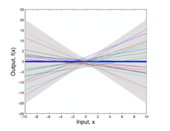
However, we are more interested in the distribution over functions induced by the distribution over parameters, rather than the distribution over parameters. We can characterize the properties of these functions:

\begin{aligned} & f(x | a_0, a_1) = a_0 + a_1x \\ \\ & \mathbb{E}[f(x)] = \mathbb{E}[a_0] + \mathbb{E}[a_1]x = 0\\ \\ \textrm{cov}[f(x_b), f(x_c)] &= \mathbb{E}[f(x_b)f(x_c)] - \mathbb{E}[f(x_b)]\mathbb{E}[f(x_c)]\\ & = \mathbb{E}[a_0^2 + a_0a_1(x_b + x_c) + a_1^2x_bx_c] - 0\\ & = \mathbb{E}[a_0^2] + \mathbb{E}[a_0a_1(x_b + x_c)] + \mathbb{E}[a_1^2x_bx_c]\\ & = 1 + x_bx_c+ 0\\ & = 1 + x_bx_c \end{aligned}

This gives the first and second moments of the function for random variables along the x-axis.

Using a little algebra, we can show that any collection of values from this set has a joint Gaussian distribution:

\begin{aligned} \left[ f(x_1) ..f(x_N) \right] \sim \mathcal{N}(0, K) \end{aligned}

where $K$ is defined by,

\begin{aligned} K_{ij} = \textrm{cov}(f(x_i), f(x_j)) = k(x_i, x_j) = 1 + x_bx_c \end{aligned}

This is a Gaussian process

Gaussian Process

A Gaussian process (GP) is a collection of random variables, any finite number of which have a joint Gaussian distribution. We write $f(x) \sim \mathcal{GP}(m, k)$ to mean

\begin{aligned} \left[ f(x_1) ..f(x_N) \right] \sim \mathcal{N}(\mu, K) \\ \mu_i = m(x_i) \\ K_{ij} = k(x_i, x_j) \end{aligned}

for any collection of input values $x_1…x_N$. Then, $f$ is a GP with mean function $m(x)$ and covariance kernel $k(x_i, x_j)$

As an example, consider Linear Basis Function Models:

• Model speficiations:

\begin{aligned} f(x, \mathbf{w}) = \mathbf{w}^T\phi(x) \end{aligned} \begin{aligned} p(\mathbf{w}) = \mathcal{N}(0, \Sigma_w) \end{aligned}

• Moments of the induced distribution over functions:

\begin{aligned} & \mathbb{E}[f(x, \mathbf{w})] = m(x) = \mathbb{E}[\mathbf{w^T}]\phi(x) = 0\\ \\ \textrm{cov}[f(x_i), f(x_i)] &= k(x_i, x_j) = \mathbb{E}[f(x_i) f(x_j)] - \mathbb{E}[f(x_i)]\mathbb{E}[f(x_j)]\\ & = \phi(x_i)^T \mathbb{E}[\mathbf{w}\mathbf{w^T}]\phi(x_j) - 0\\ & = \phi(x_i)^T\Sigma_w\phi(x_j) \end{aligned}

In this example, $f(x, \mathbf{w})$ is a Gaussian process, $f(x) \sim \mathcal{N}(m, k)$ with mean function $m(x) = 0$ and covariance kernel $k(x_i, x_j) = \phi(x_i)^T \Sigma_w\phi(x_j)$

We generally have more intuition about the functions that model our data than the weights $\mathbf{w}$ in a parametric model. We can express these intuitions using a covariance kernel. Additionally, the kernel controls the support and inductive biases of our model, and thus the model’s ability to generalize to unseen data.

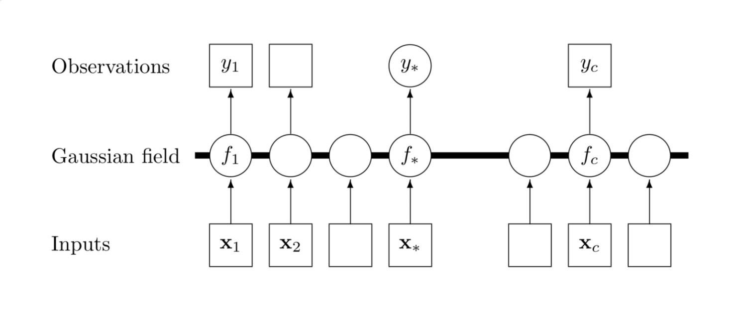
Graphical Model of Gaussian Process

Graphical Model Representing Gaussian Process

Kernel Example: RBF

RBF (Radial Basis Function) is the most popular kernel used with Gaussian processes. It is given as

\begin{aligned} k_{\text{RBF}(x, x')} &= \text{cov} \left( f(x), f(x') \right) \\ &= a^2 \exp \left(-\frac{\Vert x-x'\Vert^2}{2\ell^2}\right) \end{aligned}

• The kernel function will have high values when the two points are closer together which expresses the intuition that nearby points are more correlated in function values than farther ones.

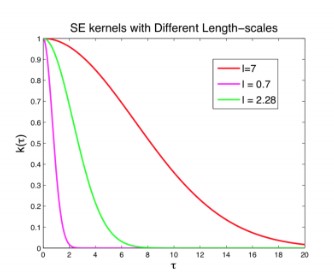
• $a$ controls the amplitude and $\ell$ controls its wiggliness, that is high value of $\ell$ will lead to higher range of distances for which the kernel gets high values and vice versa as depicted in the figure below

$\tau=x-x'$, the figure shows the values of RBF kernel with different values of $\ell$

Gaussian Process Inference

Now we study how to perform inference using Gaussian process. That is given a set of training points and their predictions, we want to compute predictions for new points not in the training set.

• The observed noisy data is given as: $\mathbf{y} = (y(x_1), \ldots, y(x_N))^T$ at input points $\mathbf{X} = (x_1, \ldots, x_N)$.

• We begin with a standard regression assumption that $y(x)$ has a gaussian distribution with mean $f(x)$ and variance $\sigma^2$, that is $y(x) \sim \mathcal{N}(f(x), \sigma^2)$

• Now, we place a Gaussian process distribution over the noise free functions $f(x)$, that is, $f(x) \sim \mathcal{GP}(0, k_\theta)$ where $\theta$ describes the parameters used to define the kernel $k$.

• Given text input $\mathbf{X}_{*}$ we can infer $f$ using $p(f_{*} \mid \mathbf{y}, \mathbf{X}, \mathbf{X}_{*})$. The joint distribution of $\mathbf{y}$ and $\mathbf{f}_{*}$ is given as

\begin{aligned} \begin{bmatrix} \mathbf{y} \\ \mathbf{f_*} \end{bmatrix} \sim \mathcal{N} \left(\mathbf{0}, \begin{bmatrix} k_\theta (\mathbf{X}, \mathbf{X}) + \sigma^2\mathbf{I} & k_\theta (\mathbf{X}, \mathbf{X}_*) \\ k_\theta (\mathbf{X}_*, \mathbf{X}) & k_\theta (\mathbf{X}_*, \mathbf{X}_*) \end{bmatrix} \right) \end{aligned}

We can condition over $\mathbf{y}$ to predict the distribution of $\mathbf{f}_{*}$ which is given as,

\begin{aligned} \mathbf{f}_* \mid \mathbf{X}, \mathbf{X}_*, \mathbf{y}, \theta &\sim \mathcal{N} (\bar{\mathbf{f}}_*, \text{cov}(\bar{\mathbf{f}}_*)) \\ \bar{\mathbf{f}}_* &= k_\theta (\mathbf{X}_*, \mathbf{X}) [ k_\theta (\mathbf{X}, \mathbf{X}) + \sigma^2\mathbf{I} ]^{-1} \mathbf{y} \\ \text{cov}(\bar{\mathbf{f}}_*) &= k_\theta (\mathbf{X}_*, \mathbf{X}_*) - k_\theta (\mathbf{X}_*, \mathbf{X}) [ k_\theta (\mathbf{X}, \mathbf{X}) + \sigma^2\mathbf{I} ]^{-1} k_\theta (\mathbf{X}, \mathbf{X}_*) \end{aligned}

This comes from a standard result over multivariate normalize distribution. Refer to this article for more information.

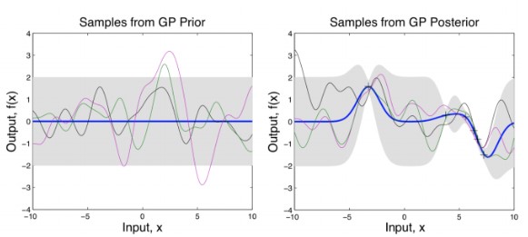
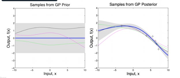
This is pictorially represented in the following two figures (with an RBF kernel). The gray region shows the variance. The left figure shows the distribution of points without any observed data points. Without any observed points, this covariance matrix reduces to $k_\theta (\mathbf{X}_, \mathbf{X}_)$, which will be same along the diagonals (Hence the same width). When some points are observed (show by x mark), the variance at those points reduces as shown in the right figure.

$\tau=x-x'$, the figure shows the values of RBF kernel with different values of $\ell$

If we increase the scale parameter $\ell$, we get a smoother looking distribution.

$\tau=x-x'$, the figure shows the values of RBF kernel with different values of $\ell$

Gaussian Process Learning

So far we covered inference with gaussian process, to learn the parameters of the kernel $\theta$, we maximize the likelihood of the observations with respect to $\theta$ by marginalizing over the entire Gaussian process $f(x)$ given as,

\begin{aligned} p (\mathbf{y} \mid \theta, \mathbf{X}) &= \int p (\mathbf{y} \mid \mathbf{f}, \mathbf{X}) p (\mathbf{f} | \theta, \mathbf{X}) d\mathbf{f} \\ \log p (\mathbf{y} \mid \theta, \mathbf{X}) &= \underbrace{-\frac{1}{2}\mathbf{y}^T(k_\theta + \sigma^2 \mathbf{I})^{-1} \mathbf{y}}_{\text{model fit}} - \underbrace{\frac{1}{2}\log |k_\theta + \sigma^2 \mathbf{I}|}_{\text{complexity penalty}} - \frac{N}{2} \log (2\pi) \\ \end{aligned}

We can use gradient descent to find a $\theta$ which maximizes this log-likelihood

Deep Kernel Learning

There are multiple ways in the literature to define kernel functions such as kernel as function of the distance (like RBF), spectral mixture kernels , kernels defined on strings/sequences, fisher kernels and so on. Recent work has introduced deep kernels,

\begin{aligned} \kappa (x, x') &= k(h(x), h(x')) \end{aligned}

where $h(x)$ is the representation of x learned using a neural network $h(.)$. These parameters $\mathbf{w}$ of $h(.)$ can be learned jointly with the kernel hyperparameters (e.g. $a$ and $\ell$ in RBF kernel) by maximizing the log-likelihood mentioned above using backpropagation through the network.

\begin{aligned} \frac{\partial \mathcal{L}}{\partial \theta} &= \frac{\partial \mathcal{L}}{\partial k_\theta} \frac{\partial k}{\partial \theta} \\ \frac{\partial \mathcal{L}}{\partial \mathbf{w}} &= \frac{\partial \mathcal{L}}{\partial k_\theta} \frac{\partial k}{\partial h(x; \mathbf{w})} \frac{\partial h(x; \mathbf{x})}{\partial \mathbf{w}} \end{aligned}

This parameterization makes it easier to apply gaussian processes on a wide range of tasks, for example, sequential data. A sequence can be encoded using a recurrent neural network and a kernel function can be applied to the encoded representation. For more details, please refer to (cite) which uses a Gaussian process on top of a LSTM to predict the prediction of lead by vehicles.

The Scalability Issue

GP inference requires computing inverse and determinants of huge covariance matrices over the entire training data which can be computationally intenstive.

• Inference requires a $(k_\theta + \sigma^2 \mathbf{I})^{-1} \mathbf{y}$ step and,
• Learning requires a $\log \mid k_\theta + \sigma^2 \mathbf{I} \mid$ step,

Both of these computation require an $\mathcal{O}(n^3)$ time and $\mathcal{O}(n^2)$ storage.

There are three families of approaches for inference

• Approximate non-parametric kernels in a ‘dual space’ with finite basis. This requires $O(m^2n)$ computations and $O(m)$ storage for $m$ basis functions. Examples: SSGP, Random Kitchen Sinks, Fastfood, A la Carte.
• Inducing point based sparse approximations. Examples include SoR, FITC, and KISS-GP.
• Exploit existing structure in K to quickly (and exactly) solve linear systems and log determinants. Examples: Toeplitz and Kronecker methods.

Inducing Point Methods

We can approximate GP through $M < N$ inducing points $\hat f$ to obtain Sparse Pseudo-input Gaussian Process (SPGP) prior: $p(f) = \int d \hat f \prod_n p(f_n \mid \hat f) p(\hat f) $

• $\mathcal{N}(0, K_n) \approx p(f) = \mathcal{N}(0, K_{NM}K_M^{-1}K_{MN} + \Lambda)$
• SPGP covariance inverted in $O(M^2N) \ll O(N^3)$, which is much faster

Running Exact GPs on GPUs

Key idea is to use a clever distributed GP learning algorithm and inference algorithms on multiple GPUs

Summary

• Gaussian processes are Bayesian nonparametric models than can represent distributions over smooth functions
• Using expressive covariance kernel functions, GPs can model a variety of data (scalar, vector, sequential, structured, etc.)
• Inference can be done fully analytically (in case of Gaussian likelihood)
• Inference and learning are very computationally costly since exact methods require inversion of large matrices
• There is a variety of approximation methods to GPs that can bring down the learning and inference cost to $O(n)$ and $O(1)$, respectively
• Many new libraries based on Tensorflow, PyTorch, Keras – despite computational constraints, GPs are certainly quite popoular

Meta-learning and Neural Processes

So far, we assume that data was generated by a single function. What if there are multiple data-generating functions, and each time we get only a few points from one of them. Can we identify it?

Definition of meta-learning

In standard learning, given a distribution over examples (single task), we learn a function that minimizes the loss $\hat \phi = \arg\min_{\phi} E_{z \sim D}[l(f_{\phi}(z))]$

In learning-to-learn, given a distribution over tasks, output an adaptation rule that can be used at test time to generalize from a task description: $\hat \theta = \arg\min_{\theta} E_{T \sim P}[L_T(g_{\theta}(T))]$ where $L_T(g_{\theta}(T)) \coloneqq E_{z \sim D}[l(f_{\phi}(z))]$, $\phi \coloneqq g_{\theta}(T)$

Examples:

• Few-shot image classification: multiple datasets, each of which includes a few examples of each class.
• Few-shot user-specific recommendation: recommend twitter posts to users; each user has different set of likes and dislikes (binary prediction)
• Contextual interpretability: interpretable linear model conditioned on images
• One-shot imitation learning: imitate a single behaviour from demonstrations; give a new demonstration, produce a policy to quickly imitate the demonstration

Conditional Neural Processes Try to produce representations for observable inputs and labels, $r$. The representations are aggregated and fed to function $g$ for prediction. So we can produce different function $g$’s given different sets of training data. This is similar to Gaussian Processes.

Attentive Neural Processes Incorporates attention mechanism into neural processes. Instead of using MLP, use attention to attend to differnt parts of contexts. Proposed based on the observation that neural processes tend to under-fit.

Summary

• There are cases when learning a single function is not enough – contextual models are used in such cases
• Few-shot learning is a popular application of meta-learning, where contextual models are trained on distributions of different tasks. Examples include solving different sub-problems, imitating different demonstrations, and making predictions about different user preferences
• Neural processes propose an alternative to kernel learning (kernel becomes fully implicity; the model is scalable without approximations)